Preventing Interactive Shells in Production Kubernetes Containers

Introduction

At Ginkgo we ensure that actions taken on software running in production are recorded and auditable. This is generally good practice and there are compliance regimes that require this level of logging and auditability.

We also want to enable our software engineering teams to easily troubleshoot their production applications. When running applications in our Kubernetes (k8s) clusters, we can use core, standard RBAC (Role Based Access Controls) and the cluster audit logs to capture actions taken on cluster resources to ensure adherence to these best practices and policies.

This blog will explain how we used OPA Gatekeeper policies to resolve tension between engineers wanting to execute shell commands in running containers when troubleshooting, while still capturing actions in the K8s cluster audit logs.

The Problem with kubectl exec and Auditability

While we hope to provide all the visibility a software developer could want with our observability tooling, sometimes instrumentation is missing. Developers understandably want the ability to execute commands within running containers when under pressure to quickly resolve a production issue.

Kubernetes provides an exec API , which allows for executing shell commands within a Pod container.

Unfortunately, once an interactive shell session is initiated, any commands issued within the container are no longer captured by the K8s audit logs. The audit logs record who issued an exec on which pod container, and that’s it.

Using standard RBAC resources we can deny any exec command entirely, but developers would feel the loss of that capability. What we really want is to prevent interactive shell sessions, to which the audit logs are blind. Standard RBAC resources are not able to differentiate between interactive and non-interactive exec calls. With non-interactive exec commands, the shell commands are captured in the audit logs. While it may slow developers to have to construct individual exec commands, they can get the troubleshooting capabilities they need while satisfying logging and auditability constraints.

What is OPA Gatekeeper and How Does it Solve the Problem?

Open Policy Agent (OPA) is an open-source policy engine. OPA Gatekeeper is built on top of OPA to provide K8s specific policy enforcement features. The Software Developer Acceleration (SDA) team at Ginkgo is responsible for operating (Elastic Kubernetes Service) EKS clusters. SDA was already considering implementing OPA Gatekeeper for a few cluster policy enforcement use cases.

When concerns about allowing non-interactive exec arose, we thought OPA Gatekeeper might provide a solution. We stumbled upon a Gatekeeper GitHub issue, which described our exact use case. This issue suggested that it should be feasible to implement an OPA Gatekeeper constraint to act on the PodExecOptions which determine whether an exec is interactive or not.

OPA Gatekeeper uses the OPA policy engine to enforce policy in K8s by defining Custom Resource Definitions: ConstraintTemplates and Constraints. Those resources integrate with K8s admission controllers to reject API calls and resources which violate a constraint. K8s admission controls are implemented using validating and mutating webhooks.

OPA Gatekeeper also provides a library of ConstraintTemplates for many common policy use cases. Unfortunately, preventing interactive exec is not one of the already implemented ConstraintTemplates in the community library.

SDA set up the OPA Gatekeeper and then started experimenting and learning how to craft ConstraintTemplates and Constraints based on the examples in the library. OPA policies are expressed in Rego, and this required some learning by members of the SDA team as it’s a Domain-Specific Language (DSL).

Enabling Gatekeeper Webhooks to Validate exec Operations

The first challenge we faced was ensuring that the OPA gatekeeper ValidatingWebhookConfiguration could validate the exec operations. Validating webhook rules match on the following API features:

  • Operations
  • apiGroups
  • apiVersions
  • Resources
  • Scope

To act on exec calls, the webhook must include the pod/exec subresource in the resources, and it must include CONNECT in the operations. We discovered that the released Helm chart for OPA Gatekeeper at the time, only specified the CREATE and UPDATE operations, and had omitted the CONNECT operation. After we modified our OPA Gatekeeper install to add the CONNECT operation our constraints were able to act upon exec calls.

apiVersion: admissionregistration.k8s.io/v1
kind: ValidatingWebhookConfiguration
metadata:
  name: gatekeeper-validating-webhook-configuration
  namespace: gatekeeper-system
webhooks:
  rules:
  - apiGroups:
    - '*'
    apiVersions:
    - '*'
    operations:
    - CREATE
    - UPDATE
    - CONNECT
    resources:
    - '*'
    - pods/ephemeralcontainers
    - pods/exec
    - pods/log
    - pods/eviction
    - pods/portforward
    - pods/proxy
    - pods/attach
    - pods/binding
    - deployments/scale
    - replicasets/scale
    - statefulsets/scale
    - replicationcontrollers/scale
    - services/proxy
    - nodes/proxy
    - services/status

ConstraintTemplates and Constraints

ConstraintTemplates contain policy violation rules, which can then be used by multiple different Constraints.

The PodExecOption which determines whether an exec is interactive is the stdin option. In the following ConstraintTemplate, the Rego rule is reviewing the PodExecOptions object passed to it from the Constraint to determine whether stdin is true or false. If true, the request will violate the Constraint.

apiVersion: templates.gatekeeper.sh/v1
kind: ConstraintTemplate
metadata:
  name: k8sdenyinteractiveexec
  namespace: gatekeeper-system
spec:
  crd:
    spec:
      names:
        kind: K8sDenyInteractiveExec
  targets:
  - rego: |
      package k8sdenyinteractiveexec
      violation[{"msg": msg}] {
        input.review.object.stdin == true
        msg := sprintf("Interactive exec is not permitted in production constrained environments. REVIEW OBJECT: %v", [input.review])
      }
    target: admission.k8s.gatekeeper.sh

The Constraint determines the objects to which the specified ConstraintTemplate should be applied and any enforcement action to take.

SDA provides namespaces for teams operating applications in the EKS clusters. Namespaces containing applications subject to constraints are labeled.

The following Constraint applies the K8sDenyInteractiveExec ConstraintTemplate above to the PodExecOptions object. It also uses a namespaceSelector to only apply the ConstraintTemplate in namespaces bearing the label. The default enforcement action is to deny.

apiVersion: constraints.gatekeeper.sh/v1beta1
kind: K8sDenyInteractiveExec
metadata:
  name: k8sdenyinteractiveexec
  namespace: gatekeeper-system
spec:
  match:
    kinds:
    - apiGroups:
      - ""
      kinds:
      - PodExecOptions
    namespaceSelector:
      matchExpressions:
      - key: <label to constrain the environment goes here>
        operator: In
        values:
        - "true"
    scope: Namespaced

Once this Constraint was in place, we tested by issuing kubectl exec commands against some test Pods in the labeled namespace with and without the stdin option (-i).

% kubectl exec -it test-679bdcc64b-gnjll -- /bin/bash

Error from server (Forbidden): admission webhook "validation.gatekeeper.sh" denied the request: [k8sdenyinteractiveexec] Interactive exec are not permitted in production constrained environment. REVIEW OBJECT: {"dryRun": false, "kind": {"group": "", "kind": "PodExecOptions", "version": "v1"}, "name": "test-679bdcc64b-gnjll", "namespace": "default", "object": {"apiVersion": "v1", "command": ["/bin/bash"], "container": "efs-csi-test-deployment-nginx", "kind": "PodExecOptions", "stdin": true, "stdout": true, "tty": true}, "oldObject": null, "operation": "CONNECT", "options": null, "requestKind": {"group": "", "kind": "PodExecOptions", "version": "v1"}, "requestResource": {"group": "", "resource": "pods", "version": "v1"}, "requestSubResource": "exec", "resource": {"group": "", "resource": "pods", "version": "v1"}, "subResource": "exec"}
% kubectl exec test-679bdcc64b-gnjll -- echo foo 

foo

(Feature photo by Nikola Knezevic on Unsplash)

Optimizing Your Docker Builds

Introduction

A few years ago, I wrote a blog post about Dockerfile optimization and how you can organize a Docker image’s layers to leverage the build cache and speed up your Docker builds. The state of the art has advanced since I wrote that blog post. BuildKit is now, as of Docker Engine version 23.0, the default build backend. The principles of how to optimally organize the layers of a Docker image are largely the same, but BuildKit introduces, among other things, fundamental improvements in caching. As I did in my previous blog post, I will use an example to demonstrate some of these improvements.

Setup

As before, we will use the official React Tutorial as our demonstration app (although the Tutorial has been updated since my previous blog post). Download the entire React Tutorial SandBox, including package.json, into a working directory. (Notice that the .js and .css files should go into a src subdirectory, and the index.html file should go into a public subdirectory.) We will be using yarn, so run npm install --save-dev yarn to install it as a development dependency. Then run yarn install to create the yarn.lock file.

We will use the same Dockerfile, though with an updated base image, as last time:

FROM node:20-alpine3.18

COPY package.json /usr/src/tic-tac-toe/package.json
COPY yarn.lock /usr/src/tic-tac-toe/yarn.lock
WORKDIR /usr/src/tic-tac-toe
RUN ["yarn", "install"]
​
COPY . /usr/src/tic-tac-toe
RUN ["yarn", "build"]

Importantly, we need to make sure that we do not accidentally COPY the node_modules (or even .git), so create a .dockerignore file:

.git
node_modules

Cache Demonstration

BuildKit is the improved backend which succeeds Docker’s legacy builder, and we will assume for the purposes of this demonstration that BuildKit is the default builder.

BuildKit offers a number of improvements to build caching, so to take advantage of caching with BuildKit, the command we run to build the image is a little bit different than before. Run this command:

docker build \
  --tag your/docker/registry/here/optimize-dockerfile:latest \
  --cache-to type=inline \
  --push \
  .

This command will build, tag, and push the image to your registry. BuildKit offers a number of different cache backends. By default only the local cache, which is the build cache on the local filesystem, is enabled. There are other cache backends which will allow us to cache our Docker builds across different CI/CD instances. Here, --cache-to type=inline is a directive to use the “inline” type of cache backend, which is where the build is cached directly in the image itself.

Now, let’s make a small change to our app. In src/App.js, change:

      nextSquares[i] = 'X';

To:

      nextSquares[i] = '+';

Before we rebuild the Docker image with our change, let’s simulate the conditions of a CI/CD instance freshly spawned with a cold cache by completely pruning our Docker environment. Run:

docker system prune -a

And enter ‘y’ when prompted.

Now run:

docker build \
  --cache-from your/docker/registry/here/optimize-dockerfile:latest \
  .

The output will look something like:

 => [internal] load .dockerignore                                                                                 0.0s
 => => transferring context: 58B                                                                                  0.0s
 => [internal] load build definition from Dockerfile                                                              0.0s
 => => transferring dockerfile: 266B                                                                              0.0s
 => [internal] load metadata for docker.io/library/node:20-alpine3.18                                             0.8s
 => importing cache manifest from your/docker/registry/here/optimize-dockerfile:latest                                  1.0s
 => [1/7] FROM docker.io/library/node:20-alpine3.18@sha256:32427bc0620132b2d9e79e405a1b27944d992501a20417a7f4074  0.0s
 => [internal] load build context                                                                                 0.0s
 => => transferring context: 487.06kB                                                                             0.0s
 => [auth] [redacted]                                                                                             0.0s
 => CACHED [2/7] COPY package.json /usr/src/tic-tac-toe/package.json                                              0.0s
 => CACHED [3/7] COPY yarn.lock /usr/src/tic-tac-toe/yarn.lock                                                    0.0s
 => CACHED [4/7] WORKDIR /usr/src/tic-tac-toe                                                                     0.0s
 => CACHED [5/7] RUN ["yarn", "install"]                                                                         35.7s
 => => pulling sha256:c926b61bad3b94ae7351bafd0c184c159ebf0643b085f7ef1d47ecdc7316833c                            0.3s
 => => pulling sha256:4b45d679ee3ef9e23a172a5bbd340012ea4515eec334cd86acf96f92ed40717a                            0.3s
 => => pulling sha256:b519384a30f5a620cfb09aa166d6c3ad7bf64b4731435d9e32153731f636a06b                            0.8s
 => => pulling sha256:095f19a54610183ae53834b1c703b05553b5bd920e6a40a38045c205569a51de                            0.2s
 => => pulling sha256:78508e7796da40c6996da8f58a1a4329f5cfcb5c6d33cfb215bdc179b4984cb6                            0.2s
 => => pulling sha256:29c1ccb5ef912ea427f74a6947a3b22bec7418df01459080c5dc13f679550453                            0.3s
 => => pulling sha256:4f4fb700ef54461cfa02571ae0db9a0dc1e0cdb5577484a6d75e68dc38e8acc1                            0.2s
 => => pulling sha256:bc11ece0c87450dfe61c56c616fc0a6413ca59938f31331e5274a7f1630869b7                            1.4s
 => [6/7] COPY . /usr/src/tic-tac-toe                                                                             0.9s
 => [7/7] RUN ["yarn", "build"]                                                                                   8.4s
 => exporting to image                                                                                            0.0s
 => => exporting layers                                                                                           0.0s
 => => writing image sha256:b48644823a4e8fb3627874214949899343d7ec48bbe06e3b0d0f0f22e6bc0147                      0.0s

You can see here that Docker loads the cache manifest from the “cache from” image (just the manifest, not the entire build cache) early in the process, and is therefore able to consult the cache manifest and determine that the first five steps of the build are in the build cache. Step 6 is not cached, the change in src/App.js invalidating the COPY command.

At this point, Docker finally does download the cached layers from the “cache from” image to use to build the remainder of the image (Steps 6 and 7). Notably, Docker only downloads the layers from the “cache from” image that it needs, not the entire “cache from” image, and we did not need to docker pull it before building.

Takeaways

Our simple demonstration only scratches the surface of the strategies and considerations for Docker build optimization. Docker offers the “registry” cache backend as a more sophisticated alternative to the “inline” cache backend, as well as other backends that are, as of this writing, experimental.

The “registry” cache backend is suitable for caching multi-stage builds, as you can set the cache mode to “max” and cache all the layers of the image, while keeping this cache separate from the image itself. We have not touched on multi-stage builds, but BuildKit introduces improvements in this area as well.

As your Dockerfiles get more complex, there is certainly a lot of room to get creative in order to keep your build processes optimal!

(Feature photo by frank mckenna on Unsplash)

Ginkgo Hack Week

Introduction

Earlier this year, we gathered in Ginkgo’s Boston HQ for Hack Week: an opportunity for the whole team to gather, to meet remote colleagues face to face, to work on passion projects, and to see just how much we can get done in a single focused week. No top-down planning and prioritization, no meetings, no tickets – just a Slack channel to coordinate, desk space, coffee, and a view of Ginkgo’s robots.

The rules were simple:

  • Meetings are canceled. Regular work is paused.
  • Everyone is free to work on anything Ginkgo-related.
  • Teams are allowed and encouraged.
  • Demo by Friday afternoon.

In this post, we’ll share some highlights of what was accomplished; some thoughts on why events like Hack Week are important; and some implementation tips to try this with your team

The Results

At the end of the week, 36 projects by teams from 1 to 12 people shared their accomplishments. The projects ranged from small quality of life improvements to existing software, to exploration of new services, to experiments with exciting new technologies. A number of the “hacks” were such clear wins that they went straight to production while others informed ongoing development and roadmaps.

To give you a taste of what the team built, here are a few brief descriptions:

  • An exploration of technologies like NFC and QR codes to streamline equipment reservations and logins.
  • Quality of life improvements by extracting code into common libraries, speeding up CI/CD pipelines, upgrading dependencies and creating bots to automate upgrades.
  • Our tools are wide-reaching, complex, and fast-moving; several projects improved the way we communicate updates to our scientists by automating the delivery of targeted, personalized messages.
  • Acceleration of the default analyses we run on every NGS sample – thousands of analyses per day – reducing the runtime by 42%!
  • A prototype for easier examination of Omics data that our HTS team creates.
  • Use of ChatGPT to create chat interfaces to complex APIs, lowering the costs and barriers to entry for exploring our data with powerful libraries.
  • Improving access to internal knowledge by leveraging “Retrieval Augmented Generation” (RAG): using a stock LLM paired with an searchable database of internal documents to answer questions.

We also took advantage of the whole team being together in Boston to have some fun with team dinners and games of giant chess.

giant chess

A post-hackweek survey of the Digital Technology department showed that the event was an unmitigated success, with 100% of the respondents calling it a good use of time (“agree” or “strongly agree” on the Likert scale).

Why Hack Week Is Important

Some folks might raise an eyebrow at an entire department spending a whole week working on… who knows what, honestly. There is no project planning, no deliverables, no scope of work! Are Hack Weeks a ZIRP?

There are 3 main reasons we believe this is a great use of our time:

  • Hack Week makes us faster.
  • Hack Week provides an opportunity for outsized returns on investment.
  • Hack Week makes us a stronger team.

Hack Week Makes Us Faster

Hack week makes us faster by fixing two kinds of friction:

  • Friction in the products and services we provide
  • Friction in tools and processes we use to develop and deliver those products and services

This is super important, because for a company like Ginkgo, speed is a compounding benefit.

Friction in Products and Services

In every organization, the folks doing the “hands-on” work – engineers, designers, help desk support agents, and others – know a ton of small problems that never quite make it into the prioritized list of issues and ranked list of projects that come out of planning processes. These might be documented annoyances, tech debt, or just that thing you saw and filed away in your brain hoping to fix that one day.

The usual way to address this is to tell teams to allocate some % of total estimated effort to fixing things like that. In practice, this is necessary but not sufficient. Some issues need sustained focus, and a few hours here and there are not enough. Some issues don’t quite feel bad enough at the moment – even if they are major time-sucks over time – to work on when there are other pressing deadlines. Some folks just feel uncomfortable going off-plan, for a variety of reasons.

Hack Week removes all that. Just go fix it! Need focus time? Have a whole week. Need prioritization? You wanting to fix it is priority enough.

Every decent-sized engineering org has people who are highly motivated by making things work better. They will fix problems whose true impact is much larger than we realize. But we must get out of their way and let fixers fix and make the tools more usable, processes more automated and make everything just a bit faster.

Friction in Tools and Processes

We aim to pull out all the friction during Hack Week – just put your headphones on, work on your thing, and ship (to a demo environment). Every time we do this, we find out that there are aspects of our setup that cause friction.

Certain operations can only be done by a few specific people, or require multiple handoffs, or occur on rigid schedules. Some things just require too much busy work and oddly specific knowledge.

Every year, we’ll find this kind of stuff – clear signs of what slows us down every week, but become obvious in Hack Week, when we are all trying to go from start to finish on a tight timeline. So we apply pressure to get things done quickly, and observe what slows people down. We take these learnings, and we improve our tools and processes. Templates get created, automation and bots put in place, conventions and status quo rethought.

We become faster at doing our jobs – in all weeks, not just Hack Weeks – as a result.

Speed is a Compounding Benefit

There’s a lot of digital ink spilled on the benefits of speed for companies in general – speed of execution, speed of innovation, speed of response to customer needs.

For straightforward end to end project delivery speed, it’s a no-brainer. There’s simple linear math here: if you can make and sell 10 widgets in the time it takes someone else to make and sell 8, you are making 20% more in the same amount of time. But it gets better. If you are 20% faster than the competition, everything else being equal, you get way more than a 20% increase in your share of the market. You might even grow the market, through speed alone, because projects that were not feasible because of the timelines become possible. Turnaround speed is a critical feature; this is why Amazon invested in their delivery network, for example.

But it gets better. Ginkgo is fundamentally not in a widget-making business, we are in an innovation and applied research business. The speed with which we iterate and learn is crucial. Faster processes and tools mean faster OODA loops and faster DBTAL cycles. Faster loops and cycles mean shorter time to learning and insights. That means we don’t just create the end product faster, we learn how to get better and faster, faster. That’s a compounding benefit.

The time we spend in Hack Week making everything work smoother and faster has a huge return on investment.

Hack Week is a Shot at Outsized Returns on Investment

Most of the year, we create project plans, interview stakeholders, write down requirements, break down and estimate tasks, set goals – the whole thing. We do this for risk mitigation and predictability. We need to know that the things we are planning to do stand a decent chance of delivering. We’ve got people depending on us! Promising more than we can deliver is bad. Running into unexpected problems and blowing deadlines is bad. Discovering half way through that you need another team to have done something, while they are completely focused on something totally different, is bad.

It’s important to do this stuff, it’s what keeps the balls in the air. Most of the time.

Planning and estimation reduce risk and improves predictability by removing variance in work outputs. Which is mostly a good thing! The problem is that reducing variance not only removes the lows, but also trim the highs. It is an approach built to minimize investments in big, risky moves, because failure is expensive.

Hack Week is the opposite. We encourage big, risky moves, and we celebrate failure. Got an idea that will make us 4x faster or easier? Go for it! It might fail. It’ll probably fail. That’s ok. It might succeed! Or it might give us great information, by failing, for how it might succeed next time!

Hack Week encourages high variance work. High variance work gives us a shot at completely changing the trajectory.

Hack Week Makes Us a Stronger Team

The hacking, learning, and social activities we organize during the week make us a stronger team, which translates to the other 51 weeks a year. By spending time working and having fun together, we are able to form stronger cross-team bonds. This makes communication and collaboration easier. By providing time to learn, experiment, and teach others, we are creating space for learning and growth, investing in the team, in our skills and success. Through social activities and mixers we put faces to names and create opportunities to see each other as real, three-dimensional people, not just slack handles and Zoom rectangles. This improves our social cohesion and greases the workings of the digital technology machine.

Rolling Your Own

Here are some tips and tricks we use to pull off Hack Weeks.

Schedule and Organization

You don’t want to introduce too much process for how people choose what to work on, but a little bit of structure helps. We create a wiki page for every hack week with a table to which people can add short idea blurbs, links to further explainers, and a list of who is planning to work on the idea and what help they need. We also create a temporary Slack channel for idea discussions a month or two before the event.

And the most important thing: we remind everyone, especially team managers, to cancel all meetings.

On Monday, we kick the week off with a quick get together to have coffee and pastries, go over the timeline, and give folks a last-minute chance to find teammates and ideas they want to pursue.

The middle of the week is spent hacking. We also organize learning opportunities – discussions on technical topics, “office hours” with internal and external experts, whatever people are into. Since we are a distributed team, and Hack Week is our one annual get-together, we also encourage folks to plan optional team activities like dinners and other outings.

On Thursday, some fraction of people always want to stay late and finish up their projects. We don’t require or expect folks to do that, but since many do, we support them by ordering pizza and feeding anyone still in the office late. Great conversations and early demos happening over Thursday Pizza are a Hack Week hallmark.

Friday afternoon is Hack Fair. We share out all the project presentations through Slack, put up posters and demos, and invite the whole company to check out what we’ve been up to. Many great discussions happen around those posters!

Riding high on the excitement of doing demos, seeing what amazing things our colleagues have accomplished, and all the stimulating conversations, we head off to an offsite and the sunset.

Presentations

One of the few Hack Week requirements is that teams do their best to present their work by Friday. To make this easier, we created a standard template for slides that can be distributed for remote viewing, or printed out and glued to poster boards for the Friday Hack Fair. The template is intentionally simple, with a slide for each of the following:

  • Project Name & list of team members
  • Big bold succinct problem statement
  • Problem context – whom the problem impacts, why it matters
  • What’s your bright idea?
  • What did you actually do?
  • State of the hack: where you got to, how can we play with it.
  • What’s next?

We found that having a standard template is good both for the hackers, who spend less time wondering what and how they are supposed to present, and for Hack Fair attendees (including other hackers!) who can read & understand standardized presentations faster.

Of course, we allow – and encourage! – live demos to go with the posters and slides.

Voting

We use Confluence templates to generate pages for each project – hosting the project presentation and any links or narrative descriptions teams want to add. Folks are invited to vote for their favorite projects during Hack Fair, and during the week after. They can vote for as many projects as they like. Voting is simply hitting a thumbs-up emoji on the relevant page. Some enterprising individuals have taken to generating QR codes and putting them on their posters, to make voting even simpler.

Keeping It Tidy

A bunch of people hacking on lots of projects can leave a lot of debris around. To minimize this, we provide several resources.

Hack Week GitLab Group

A dedicated GitLab group provides a convenient landing spot for most greenfield projects, and separates them nicely from more “permanent” work. A GitHub org or even a dedicated git repo with a folder per project can work just as well. It’s nice to be able to instantly know if the code you are looking at is from a hack week project or “for real”.

Dedicated Sandboxes

Ginkgo uses AWS accounts to enforce tight access controls and segregate application domains. Developers generally have access to resources in accounts relevant to their team, but require special approvals to gain access to other accounts. In cases where leveraging a shared Kubernetes infrastructure makes better sense, we use namespaces to achieve the same goal.

To simplify Hack Week collaboration on net-new projects for folks from different teams, we create a dedicated AWS account and Kubernetes namespace, and grant all Hack

Week participants access. This way developers can work on sandboxed prototypes without running into access restrictions, and also give us a convenient method for terminating all running processes and deleting test data after hack week is over.

Automation Joy

There’s nothing quite like going from 0 to demo in five days to highlight where a bit of automation would help us focus productively on the actual problem, rather than undifferentiated heavy infrastructure lifting. It’s a real pressure test for your developer platform!

Developer portals like Backstage are great to expose scaffolding templates and “golden paths”, but you can also make do with something as rudimentary as a Jenkins job or even a shell script. Spinning up databases and servers pre-instrumented according to company conventions, scaffolding RPC services and front-ends, hooking up to your observability tools, basic CI/CD setups to make it trivial to ship the code to a staging environment, applying your company’s color palettes and design standards – automating any and all of this away for the common cases speeds up Hack Week work, and makes regular work faster and easier, too.

To Sum Up

Hack Week is a fun and exciting event where teams get to work on cool and creative projects that can lead to big rewards for the company.

Hack Week makes us faster because it gives us a chance to fix problems that needed to get addressed for a while, but have not gotten the attention they deserve. It improves our products and services. It also helps us identify what’s been holding us back and gives us a chance to fix it. The freedom to take on “high variance” work sets this week aside from all other weeks, and provides a counterweight to more sure, lower variance work we do normally.

Lastly, it’s a time when people can come together, break down barriers, and work on projects they’re passionate about. Plus, it’s a great way to bond with your colleagues and build stronger relationships.

We had fun with this one; hope you give it a try!

(Feature photo by Caspar Camille Rubin on Unsplash)

2023 Digital Tech Summer Internships: Part 3

We conclude this year’s series on our Digital Technology Interns with the cool things that Ariel and Rohan did this summer!

Ariel Fuchs, Software Engineering Intern

Introduction

Hello! I am Ariel and I am a returning software engineer intern at Ginkgo Bioworks. This summer I was placed on the Digital Tech team called Samples Genomes and Strains (SGS). SGS oversees our Laboratory Information Management System (LIMS) which is where we store information regarding samples, their location and their biological content. Sample location management is crucial as it represents where the physical samples and containers live (so researchers know where to find them) and information involving their change history or lineage. I worked mainly on a project that oversaw the location management of containers, where containers are any physical entity that can hold information (i.e. test tube, well-plate, freezer etc).

Project

Problem

For my intern project, I was tasked with revamping our container import process. The import processes on LIMS allow our scientists to create or update information in bulk. Currently, users have to copy and paste a CSV file and click run in order to import their information. The component works great when there are no formatting or value errors to begin with. However, even one mistake with the formatting or the values provided will cause error messages to be displayed. Yet even the error messages present its own challenge.screenshot of legacy LIMS container import

screenshot of legacy LIMS container import error

screenshot of legacy LIMS container import result

The first problem is that each error is displayed in its own text card. This takes up too much space if there are multiple errors. Second, the data users provide to import does not currently get reformatted to ease the process of editing. Users have to meticulously go through each row to find the right field to correct. Any change to the text input can result in new formatting errors that the user now has to correct without invoking any more. Lastly, the user has no method to check that their information is correct without submitting it in the process. So although the old way is functional, it doesn’t provide a clean user experience and can be frustrating to work with.

LIMS container import 2.0 diagram

Solution

The biggest change to the Import Container Process was splitting up the steps to input, validate, and import the data.

Step 1: Entering Data. Users can now directly upload their CSV which can mitigate any formatting errors which arise from copy and pasting. If there are any formatting issues, these issues will be presented at the top of the page.

LIMS container import step 1 screenshot

Step 2: Validate Data. Users will see their data reformatted into a table that they are able to edit or delete information. Users can validate their data and still make changes before they import the information. Any errors will prevent the user from importing their containers, but they can be easily resolved in this step. Error messages will appear both at the top of the page and at the table level so it is clear what needs to be corrected. Both the validation and import buttons rely on new GraphQL mutations that I created.

LIMS container import step 2 errors screenshot

LIMS container import step 2 success

Step 3: When users have successfully imported their data, a list of the new ids created will be displayed. Users can then find more information about their containers by clicking the links on this success page or looking through the Container View dashboard elsewhere on LIMS.

LIMS container import success screenshot

In addition to these changes, I created multiple tests to ensure that these mutations would catch any data entry errors. The new Import Container process has clear visuals, intuitive steps, and creates an overall streamlined experience for Ginkgo’s scientists. This will now be the template to improve the other import processes mentioned in the beginning of this post.

Conclusion

I gained many valuable skills this summer – learning how to create my own routes, GraphQL mutations, building different data structure views, and how to be resourceful when resolving problems. I have Yasmine Karni to thank for this successful summer as she is truly the best mentor. She created a strong learning environment, gave me freedom to explore my project, and frequently gave insightful feedback. In addition, I really appreciate the SGS team for being so supportive and encouraging. Lastly, a big shout out to the Early Talent team and the intern cohort. I loved the trivia nights, Early Talent Career sessions, and our BioDesign Presentation Competition! Working at Ginkgo Bioworks has given me two phenomenal summer experiences and insight into the software development world. I am thrilled to continue pursuing this career after my Master’s program at MIT in Computer Science and Brain and Cognitive Science. Thank you Ginkgo for helping me grow both professionally and personally, and I can’t wait to see how they change the world next!

Rohan Chhaya

Introduction

Hi! My name is Rohan and I’m pursuing my Bachelors in Bioengineering and my Masters in Data Science concurrently from the University of Pennsylvania. This past summer, I worked on the Design Center team, previously called the Terminators, to build out a new fullstack feature in Loom, Ginkgo’s platform for designing and ordering DNA. I appreciate everyone on the Design Center team for dealing with my endless barrage of questions as well as the users of this project. Big shoutout to my manager, Ashish Addepalli, and my mentor Luísa Galhardo, whom I bombarded with code review requests every single day.

Project

The goal of my project was to create a feature where users can mark certain DNA as a positive control, which is a benchmark that is known to produce an expected outcome in an experiment. Based on the number of DNA constructs being ordered, a certain number of replicates, or copies, of these controls would be added to the transaction and randomized on the plate. This end-to-end feature allows users to easily customize their experiments with controls while abstracting away the tediousness of remembering and replicating certain DNA controls.

Designing Control DNA Constructs

Users can already use a variety of tools, like the drag-and-drop workspace, to organize various pieces of DNA. These pieces are called “design units” and live in categories called buckets, like a promoter bucket for DNA that initiates gene transcription. In any given experiment, certain design units may be added to the design to be used as a positive control sequence. These design units can now easily be marked or unmarked as positive controls, complete with buttons and visual icons. Next, users create constructs by assembling together in a combinatorial manner (for example, 2 buckets with 2 design units each → 4 constructs). Any construct that has a design unit that was marked as a positive control automatically inherits this positive control designation.

DNA controls screenshotconstructs screenshot

The design units (left) can be marked or unmarked as control, and the constructs created from them (right) inherit the designation. For example, Design Unit A is part of the top construct.

Adding to Transaction and Calculating Replicates

When the design is ready to order, users can create a transaction that has all the constructs in the design. On the transaction page, the control constructs float to the top for easy visualization in large transaction sizes. Based on data collected from the High Throughput Sequencing team, we can calculate how many replicates to add to the transaction. I designed an informative card explaining the math and links to the relevant design/design unit used to define the controls. When the user is ready to place the order, there is a pop-up confirming the new transaction size.

transaction screenshotreplicates screenshot

Ordering and Randomizing

To execute an order, we use another internally developed software called Orderly, which automates all DNA ordering with some of our vendors. Within Orderly, we can check to see if the order has positive controls and if so, we randomize the molecule ordering on the plate before placing the order with our vendors. This helps improve the blinding of the experiment, since the locations of the positive controls should be unknown to the biologist working with the plate.

My Ginkgo Experience

I had a blast this summer at Ginkgo! As someone with a background in biology and computer science, it was really cool to mix those two worlds together and work on a meaningful project that people were looking forward to using and is now in production.

I was able to improve my technical skills by working in languages and frameworks that were brand-new to me. Thanks to some of the intern events put together by the Early Talent team, I even had the opportunity to chat with upper-level executives about Ginkgo’s business strategies and the broader biotechnology industry.

Outside of the office, I had so much fun exploring Boston with my fellow interns, from kayaking on the Charles, to restaurant-hopping in Chinatown, to exploring Cape Cod. I’m very grateful to everyone who made my summer one to remember!

Conclusion

It has a been a great summer and we wish Digital Tech Team Interns well. Thank you for your impressive contributions and we hope that you have a great year!

(Feature photo by Saiph Muhammad on Unsplash)

2023 Digital Tech Summer Internships: Part 2

In our last blog post, Roshida and Sean told us about their summer internships with the Digital Tech Team at Ginkgo. This week, Himanshu, Arijit, and Hunter tell us about their internship projects!

Himanshu Reddy, Software Engineering Intern

Hey! My name is Himanshu, and I had the privilege of interning with the Lab Data Processing team this summer. I’m currently a rising senior studying Computer Science at the University of Texas, with a focus on applications to biology. I believe that there is a lot of potential to apply computing to biology, spanning applications from lab automation to AI-driven DNA design. What excites me about Ginkgo is their effort to apply robust engineering practices to biology; it’s a hard challenge, but one worth solving!

During this internship, I built a registry for Ginkgo’s custom analyses. Custom analyses are scripts written in Python and they allow us at Ginkgo to run custom processing logic on raw bioinformatics data (e.g. counting the number of barcodes in the data from a NGS sequencing run). Existing custom analyses can be made available in Servicely, our portal for foundry services.

analysis options screenshot
A page showing some of the custom analysis options available to run. The first analysis is obfuscated to protect sensitive data.

However, we didn’t keep track of what custom analyses existed at any given time and what revisions were made to them afterwards. This led to several problems, such as a lack of backwards compatibility and a tedious update procedure when adding or modifying a custom analysis in Servicely. I joined Ginkgo during an ongoing effort to fix many things affecting the custom analysis infrastructure and Servicely. My project, termed the Custom Analysis Registry (CAR), was a part of this larger effort.

I created a Django app that, essentially, keeps track of registered custom analyses. The registration process was handled using a Gitlab CI/CD pipeline in the CAR that could be imported and used in a custom analysis. Once that was done, the pipeline would make a request to register the custom analysis to the registry. The CAR would also do some prep work to set things up in AWS Batch, allowing us to run custom analyses on-demand. This allowed us to keep track of the custom analyses at Ginkgo and make the custom analysis development process much better!

custom analysis registration flow
The flow of custom analysis registration.

My internship was a very enjoyable experience! I was lucky to work with smart, motivated, and supportive people who helped and advised me during my internship. The people team also hosted many great events for the interns, like the tour of the DNA synthesis facilities in Ginkgo’s Cambridge office.

One thing I liked about Ginkgo as a whole was their open and collaborative culture. Because of it, I was able to attend many of the office hours sessions hosted by different teams. I was also excited to learn about the deep learning initiatives happening at Ginkgo, as deep learning in biology has really taken off in the past few years. I’m excited to see how biotech companies like Ginkgo incorporate AI into their workflows.

Overall, my internship was a great experience and I’d highly recommend Ginkgo Bioworks as a place to work!

Arijit Nukala, Software Engineering Intern

Hello! My name is Arijit, and I’m a rising senior at Johns Hopkins studying Biomedical Engineering and Computer Science. This summer I worked on the Operator Guide team, which owns Ginkgo’s in-house user interface for managing laboratory tasks. My project involved building a “Pause State” for Ginkgo’s lab operators.

In the lab, operators execute on the workflows that underlie specific Ginkgo Foundry services. Each workflow involves a different instrument and process. Understanding how long each of these processes takes is essential to efficient planning of Ginkgo’s projects. The goal of my project was to support the ability for an Operator to pause work after it has been started in order to more accurately calculate the turnaround time (TAT) for Ginkgo’s services. Operators needed a way to pause this clock so that requests that are blocked because of things outside the Foundry’s control don’t artificially inflate the turnaround time for the service.

For my project, I developed a Pause Annotation model and API for manipulation of data in Django, a common and powerful Python web framework that integrates with front end systems such as Ginkgo’s React based Portal-UI. The data model I created links to workflows being processed by Operators and tracks the pause time and pause reason each time work is paused. When a workflow is resumed, the resume time is also logged. Because each pause/resume for a workflow is stored in the data model (similarly to lap times on a stopwatch), we can calculate the total pause duration and working duration. All of the working or unpaused times can be added together to get the TAT for a workflow.

Originally, I planned to implement a more general “annotation” feature. Each annotation corresponded to either a “pause” or a “resume” action , and was generalizable for annotation features beyond pause/resume in the future. However, calculating TAT from data structured as two entries for each pause/resume cycle is complicated and computationally intensive. I instead opted for one entry that contains the pause and resume datetime to simplify TAT calculations later.

At the end of my internship, I was able to release my feature company wide and received positive feedback on it. I added additional features as part of an MVP+ release, presented my work to Ginkgo’s foundry teams, and created a Tableau dashboard to visualize pauses in batches. My feature had a greater impact than I could’ve imagined was impactful despite my short stint as a developer.

Being part of the Operator Guide team this summer was an amazing experience. I had a chance to see how software development teams ideate, organize, and execute their work. During my daily work and through feedback, I learned about intelligent software design, system efficiency, and the amount of teamwork that goes into designing great software.

I’m grateful for the opportunity to stay in Boston this summer and work in Ginkgo’s incredible Seaport-based office. Besides consuming enough cold brew and blueberry cobbler protein bars to last me a lifetime, I had a chance to meet other like-minded interns, develop friendships with Ginkgo employees, and enjoy Ginkgo’s fun-spirited work culture. Making biology easier to engineer through software while having a little fun along the way was a dream come true for a biomedical engineer and computer scientist like me.

Hunter DeMeyer, DevOps Intern

Introduction

Hi! My name is Hunter. I’m a graduate student studying Bioinformatics at the University of Illinois. This summer I joined the Cloud Infrastructure team to gain experience in operations so that I will be better equipped to build end-to-end solutions for scientific problems. I worked on two projects while at Ginkgo: a data visualization and business intelligence tool for surplus cloud spending and a Large Language Model for classifying DNA sequences.

AWS Cost Reduction

First, AWS cost reduction. At Ginkgo, we give our science-oriented teams a lot of freedom when it comes to provisioning the resources they need to get their work done. This lets each team independently build infrastructure as required which is great for keeping projects on schedule; however, sometimes the resources chosen are overkill for the task at hand or the resources are not shut down when they are no longer needed. Complicating things further, we follow AWS’s recommendation of using sub-accounts to isolate different workloads and enhance security. With hundreds of AWS accounts serving different teams, wasted dollars were extremely hard to track down across our entire organization.

Luckily, AWS provides a partial solution for this problem in the way of Trusted Advisor Reports. Each report focuses on a specific service and a specific optimization for it, such as cost or security. Our top interests were in Low-utilization EC2 Instances, Underutilized EBS Volumes, and Idle RDS Instances. These reports are specific to each account.

My project provides a cloud-native method for extracting and visualizing Trusted Advisor Report data. On a regular schedule, an AWS Step Function runs a lambda to log in to each AWS account and pull its Trusted Advisor Reports in parallel. These reports are then paired with some additional account information and certain fields are parsed into the proper format. From there, the step function kicks off an AWS Glue crawler to pull the reports into a Glue database. Finally, an Amazon Quicksight dashboard renders the data into interpretable and interactive visuals.

AWS cost reduction project architecture

This solution provides Digital Operations management with weekly insights into resources where spending could be optimized, so they can quickly be shut down. On the Cloud Infra team we believe that nothing should be deployed manually, so we try to automate everything as much as possible and in this case it means creating Infrastructure as Code (IaC). The entire stack of lambdas, schedulers, step functions, databases, and analyses can be recreated within minutes from an AWS Cloudformation template.

This internally developed observability platform is exciting in its own right, but it can be expanded to offer so much more in the future. In addition to visualizing data, it could also leverage the existing event-driven infrastructure to cull over-provisioned resources without human intervention, automatically keeping our cloud infrastructure as lean as possible. I’ve also written some code to downsize or terminate EC2 and RDS instances. Right now it needs to be manually triggered but eventually we’d like to have an event-driven process that can automatically reduce costs using this method. Maybe a future intern project!

While I found my Cloud Infra role rewarding, it was not as close to the science as I would want to be in a long term role. My manager Dima Kovalenko was kind enough to let me explore some of the scientific work going on at Ginkgo through a collaboration with our Vice President of AI Enablement Dmitriy Ryaboy.

AI-powered DNA Sequence Buildability Classification

One core tool we use at Ginkgo to engineer biology is DNA synthesis. Sometimes this process is straightforward and DNA fragments are easy to produce, but other times synthesis isn’t yet possible and will not be attempted. We use certain heuristics to analyze every piece of DNA requested for synthesis, and determine whether it will be buildable.This is a great example of a binary classification task, and is one that we have a ton of good-quality data for. Moreover, we have data on why sequences get rejected, as well as the relatively rare DNA sequences that our checks pass but fail to synthesize correctly. This dataset is a good candidate for experimenting with Large Language Models for biology, and comparing them to current processes in use at Ginkgo.

Large Language models (LLMs) work by “tokenizing” inputs; grouping frequent sets of symbols together and counting the number of occurrences of each one. Generalized LLMs (think ChatGPT) have a high number of symbols, and operate on relatively short sequences of text. Biology is different though; the diversity of a sequence is much lower with an alphabet cardinality of only four. Additionally, biological strings can extend to be millions of bases long. Until recently, these requirements exceeded the capabilities of LLMs. We need a specialized model that is both sensitive to individual bases and able to handle extremely large contexts.

HyenaDNA is a recently proposed LLM for biological string analysis. It replaces the usual transformer architecture of LLMs with “hyena” layers. Hyena forgoes the traditional attention mechanism, replacing it with a subquadratic convolution-based technique. This enables much longer sequences or much larger token sets. HyenaDNA takes advantage of these layers to dramatically increase the maximum possible length of an input sequence all the way to one million characters. We decided to experiment with HyenaDNA and see how well the pre-trained model performs on the buildability classification task, using both fine-tuning and in-context learning.

We have a huge amount of historical buildability information; the most difficult part of this task was extracting those data from our databases and formatting in a way that made it possible to ingest into the model; DuckDB was super helpful for this. In addition to that, we needed to ensure that the training data was not skewed to favor a particular time frame, organism, or error class. For this I had to compute a joint probability distribution that weighted each sample based on the rarity of its fields. Once the data was prepared, I stood up a powerful EC2 instance and fine tuned the hyenaDNA mode, achieving about ~80% accuracy in preliminary tests. I wish I had more time to work on this, but I’m very happy with the progress I made on it.

Final Thoughts

I had an incredible summer at Ginkgo and learned so much about being a DevOps engineer. I now know that it isn’t what I want to do long term, but am excited to apply the skills I’ve learned in future roles. I’m extremely grateful that I got to explore such a wide breadth of work at Ginkgo. I’m also very appreciative of the hard work put in by the Early Talent team, who organized tons of fun and informative events throughout the summer. Some highlights include a Boston Red Sox game, an Ask-Me-Anything session with CEO Jason Kelly, and a trip down to Cape Cod. Every bioworker I interacted with over the summer was excited about the intern program and more than happy to provide some help or just answer questions. The passion people have here is unparalleled, and I consider myself lucky to have been a part of this company for the past three months.

(Feature photo by Saiph Muhammad on Unsplash)

2023 Digital Tech Summer Internships: Part 1

It’s that time again! Our Digital Technology Team interns have wrapped up another successful summer. This is the first in a three-part series where our interns tell you about their work. We start with Roshida and Sean.

Roshida Herelle, Product Design Intern

Introduction

Hello! My name is Roshida and I am a rising Junior pursuing a Bachelor’s Degree in Technology and Information Design at the University of Maryland, College Park. This summer I have been working as a Product Design intern on the Product Design team!

Project

My summer project was to create the interface for a plate repository that scientists can use to identify and learn about the plates they use for their experiments.

A scientist's gloved hand holds a 96-well plate with a colorful array of samples
This is a 96-well plate.

Plates are used to hold samples and are arranged in grids that contain wells. Plate characteristics, such as well number, well bottom shape, maximum well volume, etc., can be influential to an experiment because they can affect things like microbial growth, liquid transfers, and other processes. This means plates can vary in a lot of different ways. At the moment, there isn’t a centralized location to see these characteristics or understand the differences between plates. Additionally, the naming schema of plates isn’t helpful to scientists because it’s inconsistent across plate types and lacks important information to guide scientists in their plate selection. Since this project will continue to develop after my internship, I was given the task of creating a new naming schema and foundational UI that will be expanded upon. I collaborated closely with Sean Doyle, a Software Engineer intern, who worked on coding the database and creating the API for the repository.

Double Diamond Method diagram
from “How to apply a design thinking, HCD, UX or any creative process from scratch” by Dan Nessler

My design process followed the double diamond method. This approach helps us thoroughly understand design problems in order to brainstorm innovative ideas and deliver a satisfactory product solution.

Through discovery user interviews, we found that scientists use external resources, such as manufacturer sites and Google spreadsheets, to find information about plates since they don’t have a single source of truth for plate types and their details. Additionally, the inconsistent plate naming schema confuses scientists because they’re not sure if what they’re selecting actually matches a plate in the lab.

generic plate name diagram
A generic name in LIMs could apply to multiple plate types in the lab. How do we make sure scientists are choosing the right plate and having that reflected in their workflows?

After conducting this research, our defined problem statement was that the current plate selection process requires a lot of mental and physical labor from scientists because their decisions are not thoughtfully guided.

Taking these findings, I brainstormed some design solutions and low fidelity screens that I brought to the team for feedback. Our main solutions were to 1) standardize the naming schema to be consistent and informative 2) create a way to filter beyond automation choices 3) show users which plates are similar and different 4) allow the automation team to onboard new plate types into the repository. We wanted this tool to be accessible through the software tools that we’ve built at Ginkgo to enable scientists to access the repository whenever possible.

sketches of plate repository UI
My initial sketches showing the search results page and plate details page.

While brainstorming naming schemas, I conducted a closed card sort. A closed card sort is a user research method where you have participants group cards into predetermined categories to better understand their mental models. In this instance, the cards were plate characteristics and the categories were “need to know in a name”, “nice to know in a name”, “don’t need to know in a name”. After testing different naming schemas, we settled on including well #, manufacturer, brand, well bottom shape, volume, and part number because users felt that it was descriptive enough to visualize and locate it in the lab.

new naming schema
Examples of the new naming schema.

Afterwards, I created user flows and sitemaps to guide my information architecture and interface design. I developed mid fidelity screens that I tested with users to get feedback.

plate repository mid-fidelity mock
Users felt like the table was overwhelming at first, so I reserved that for the additional information page. Additionally, calls to action weren’t as noticeable and users were not utilizing the filter feature as much as I hoped. They also wished the tags were more prominent.

Using their feedback, I mocked up the following high fidelity screens that were iterated on after another round of testing.

plate repository high fidelity mock 1
Upon opening the repository, the user is met with a list of characteristics they can select from. This guides their search by giving them a point of reference to start with.

plate repository high fidelity mock 1

plate repository high fidelity mock 3
I wanted to enable a grid view option for those who are visual learners as well as a list view for people who want a more condensed view of their results. Both versions have limited information/text to prevent information overload.
plate repository high fidelity mock 4
This is the plate details page that users can see upon clicking the information icon. I used drop down arrows so that users can reveal or hide as much information as they desire!
plate repository high fidelity mock 5
I designed a comparison tool for scientists to use to see the differences and similarities between plate types.
plate repository high fidelity mock 6
I designed a page for automation to use when onboarding a new plate type into the repository. I wanted automation to go through the same experience of selecting characteristics of a plate rather than typing it in to make the onboarding process faster.

End Result

My initial design solutions weren’t perfectly executed at first, and required a lot of iterations and testing to figure out an interface that wasn’t only satisfactory to myself but to the scientists who will eventually interact with this tool. Overall, I’m satisfied with the end result! Scientists found my final mockups and naming schema to be intuitive, informative, and believed it would help speed up their processes of finding a plate.

Ginkgo Experience

Though I spent a lot of time working on my project, I made sure to have some fun as well! Thanks to our Early Talent event coordinators Eddie Kaikai, Angela Perkins and Casey Wheeler, I was able to partake in intern bonding events like the Red Sox game and Intern Trivia Night. I want to give a BIG shoutout to Cynthia Pollard and Hanna Tseng for being the best mentors throughout my time at Ginkgo and making me feel supported the entire way. I also want to thank the Product Design, Product Management, Software Engineering and Automation teams for their contributions to this project and their willingness to help me bring my design vision to fruition! It was amazing to work on such a high impact project for my first internship and I can safely say I’ve developed irreplaceable skills that will help me grow as a Product Designer and individual. If I could pinpoint where I’ve grown the most, it was certainly at Ginkgo!

Sean Doyle, Software Engineering Intern

Introduction

Hello, my name is Sean Doyle and I am a rising senior at New York University studying Computer Science. I spent the summer working on the Automation Integration team as a software engineering intern and got a chance to apply my previous software engineering experience in robotics, AI, and embedded systems to the new domain of lab information management within automation! Big shoutout to Vichka Fonarev, my mentor for the summer, who helped tremendously with not just my project but also my personal growth and learning!

Main Project

Problem Statement

My main project for the summer revolved around a critical piece of labware called a “plate”.

well-plate

Plates are made up of a number of wells that store samples as they are processed through a biological procedure. They are the most important piece of labware that scientists across Ginkgo use to run their experiments and over 500 plate types have been onboarded at Ginkgo to accommodate a wide range of applications. With that said, information on the characteristics and automation compatibility for each plate type is siloed across services and people making it difficult to retrieve. This information is critical to different users, ranging from a method developer choosing a plate type that works with the proper automation, LIMS (Lab Information Management System) setting up a container with the correct plate type name and number of wells, or an automation engineer onboarding the dimensions of a plate type onto a new liquid handling robot. An inability to find these characteristics on a plate can cause critical issues such as assay failure from plate type and automation instrument incompatibility, operator confusion from vague plate type names, or automation crashes from imprecise plate type measurements. My project for the summer was to develop a service to solve these problems regarding information retrieval on plate types.

The Solution

The solution I developed is called the Labware Repository Service (LRS). It is a centralized single source of truth database that holds critical information on plate type characteristics and can integrate across platforms at Ginkgo.

labware repository service ERD
Entity relationship diagram for the LRS database.

The LRS is a backend service configured with a parameterizable API that can interface with user facing applications. The most important of these applications is the Plate Repository User Interface(UI) which is a front end service that fellow intern Roshida worked on this past summer. The Plate Repository UI allows method developers and operators to filter through the LRS database to find the right plate for their procedure. The filtering options include a number of characteristics ranging from, number of wells, automation compatibility, color, well volume and much more, all of which are stored in the LRS database. Furthermore, the LRS API provides a way to enter a new plate type, validate the entered characteristics, and ensure that duplicate plate types are never created. These features will be critical to ensuring data integrity as users interact with the LRS through the Plate Repository UI.

A number of different technologies were chosen to implement the LRS. PostgreSQL is the standard database management system at Ginkgo so it was used alongside SQLAlchemy to create the database models. Since the primary user of the database is the Plate Repository UI, GraphQL was chosen as the main API endpoint to access the database as it interfaces well with React UI applications. Additionally, GraphQL is a unified standard that other internal Ginkgo tooling uses so future integrations can easily accommodate the LRS as first party data. A set of REST endpoints were developed to interface with embedded systems in automation that cannot easily send GraphQL requests. Docker was used to containerize the LRS to make both deployment and development across platforms easier. The LRS was deployed on AWS Elastic Container Service (ECS) alongside the PostgreSQL database which was deployed on AWS Relational Database Service (RDS) both using infrastructure as code.

labware repository service architecture diagram
Architecture diagram for the LRS.

Impact of Work

There was a lot of ambiguity and conflicting information surrounding plate types which made this project difficult but rewarding. I got the chance to contribute to the product development team’s user interviews and it was illuminating to see just how differently people thought about plate types across the company. For example, an automation engineer needs to know precise plate dimensions to enter onto a robot, operators need to know about plate opacity for optical density readings, and method developers need to know how many wells a plate has so they can test their samples efficiently. Everyone’s perspective was valuable so I continuously looked for feedback on my planned database designs to meet all users’ needs with the simplest solution possible. Almost everyone I talked to mentioned how impactful the LRS would be to standardizing information about plates and was excited that someone was finally taking on the challenge. From reducing downtime due to operator confusion, to promoting automation and work cell adoption, to expanding the capabilities of automated instruments, the information stored in the LRS will impact a diverse set of users. It was humbling to be entrusted with such an important project that had far-reaching implications across Ginkgo. Additionally, this project was one of my team’s first exposures to GraphQL so it felt particularly meaningful to learn this new technology alongside my team and then contribute to my team’s shared understanding of it. Building a service from the ground up was satisfying especially knowing how expansive it was to become in the future as it integrates across existing integral services.

My Ginkgo Experience

This whole summer was a blast! During an intern event a presenter said that Ginkgo likes to hire “smart friendly people” and that really resonated with me. Whether it was shadowing operators in the lab, biking 35 miles one Sunday with a few other interns, or just random check-ins from my team offering to help me out or support my learning in any way they could, I felt like I was surrounded by role models throughout the summer. To me, the people I’m with are the most crucial factor for how impactful an experience is and rarely have I been surrounded by as many strikingly intelligent yet genuinely kind people as I have at Ginkgo. I’m very grateful for the summer I got to spend here and look forward to more memories with the lifelong friends I’ve made here!

internship fun times 2 internship fun times 1

Thanks for reading! Next time on GinkgoBits, Himanshu, Arijit, and Hunter will tell us about their summer!

(Feature photo by Saiph Muhammad on Unsplash)

Building Battle-Hardened Defenders

Background and Introduction

To clarify any misconceptions, let’s begin with some definitions. Penetration testing is a well-known concept among tech professionals. It aims to identify as many vulnerabilities as possible, assess their exploitability to demonstrate real-world impact, and report them for remediation. Red Teaming, although sharing some similarities and overlap with penetration testing, has a distinct objective. Rather than uncovering all vulnerabilities, a red team engagement emulates a real-world attacker to evaluate the blue team’s (the defenders) ability to detect and respond to an attack. Although both terms are often mistakenly used synonymously, they each serve unique purposes in offensive security testing. In essence, penetration testing focuses on assessing defenses, while red teaming evaluates the defenders. We can identify weaknesses through red teaming and better prepare our defenders to face real-world threats.

How It Works

So, how do we run a red team engagement? There are two primary approaches to consider. The first mimics a real hacker’s strategy, starting with reconnaissance, selecting a target, and attempting to gain initial access to the network. This access is often achieved through a simulated phishing exercise, where the red teamer deceives a user into downloading and executing malicious code, granting the attacker network access. However, this process can take weeks, as it relies on the phishing attempt’s success.

The alternative approach is the assumed breach methodology, which presumes that an attacker has already infiltrated the network or gained initial access. In this scenario, the tester begins with existing network access. A common way to bridge the gap between these approaches is to run a phishing campaign simultaneously with the assumed breach, allowing the assessment of initial access and social engineering aspects without waiting for the phishing attempt to succeed before proceeding with the test.

What does the engagement entail? Most red team engagements utilize Mitre’s ATT&CK (pronounced “attack”) framework to emulate the tactics, techniques, and procedures (TTPs) of an attacker. We can use ATT&CK and the ATT&CK Navigator to model threats specific to certain hacker groups and industry-specific threats. Again, when red teaming, we try to emulate a real-world attacker as closely as possible, not enumerate all vulnerabilities. Since our goal is to test our defenses and our blue team, we heavily emphasize stealth and defense evasion. By doing so, we can identify gaps in our detection and response capabilities and better counteract those techniques for the future. Many TTPs can be automated using commercial tools such as cobalt strike or open-source tools such as Mitre Caldera. The red teamer will select a target within the organization and move through the TTPs to get there.

Blue teamers should practice what is known as defense in depth, meaning if one defense fails, there should be another layer of security to prevent the full attack from succeeding. So we evaluate the detection and response capabilities throughout each engagement phase. Suppose the red team successfully can move through various TTPs undetected, or with no response by the blue team. In that case, the red and blue teams will work together to identify the gaps that allowed them to go undetected and then improve upon them. Suppose the defenders successfully detect and prevent an attack. In that case, the red team can go back and try another method to evade the defenses of the blue team. This cycle could repeat in an infinite game of cat and mouse. The result should be a comprehensive report of the strengths and weaknesses in the detection and response capabilities of the organization. Once the red teamers are satisfied that they have done this, the engagement can conclude, and they select a new target and begin to plan another engagement.

How We Utilize Red Teaming at Ginkgo

At Ginkgo, our VAPT (Vulnerability Assessment and Penetration Testing) team adopts a comprehensive approach to vulnerability assessments that extends beyond traditional penetration testing. To maximize the effectiveness of our red team capabilities, we employ cyber-war games as a powerful tool. During these war games, we embrace a “purple team” approach, leveraging the strengths of both our red and blue teams. Through close collaboration, the red team strategically progresses while the blue team’s detection and response capabilities are continuously evaluated at each phase. These exercises serve as valuable learning experiences, enhancing the capabilities of our red and blue teams. This symbiotic relationship ensures that our offensive and defensive teams have a deep understanding of each other, fostering a strong and cohesive security infrastructure.

Conclusion

We can go beyond what a traditional penetration test includes through red teaming. While it is crucial to discover and patch vulnerabilities, it is often said that “prevention is ideal; detection is a must.” In the event that things slip through our systems, we must equip our blue team for early detection and response. While performing adversary emulation, we “battle harden” our blue team defenders. While blue teamers are guaranteed to see many threat attempts in their careers, they will never experience them all, especially in the wild. By mimicking the TTPs of our industry and organization’s most likely attack scenarios, we help prepare our defenders to detect and respond to real-world scenarios.

(Feature photo by Jachym Michal on Unsplash)

Even More Rapid Retrieval from Very Large Files with Rust

Introduction

In a previous post Rapid Data Retrieval from Very Large Files, Eric Danielson discussed how Ginkgo’s software engineers are enabling fast access to massive sequence datasets. As a bioinformatician, I need file formats such as fasta and gff, for command line tools and biological sequence-processing libraries. However, these flat-file, semi-structured formats don’t scale to hundreds of millions of sequences. File compression makes data storage tractable, but finding and extracting a specific sequence among millions in a random position in the file has been a bottleneck.

Please read Eric’s full article, but the gist is that the block gzip (BGZip) from the samtools/htslib project is the highest performing tool for getting (compressed) data out of a standard file store. BGZip’s “trick” is to concatenate multiple gzipped files together – where a single gzip block is no more than 64KB. A secondary index file, under GZI extension, is used to keep track of the locations of the blocks, with respect to the compressed and uncompressed bytes. BGZipped data is itself a valid gzip archive and thus, can be (de)compressed with any gzip library.

Using these tools, we can retrieve a sequence somewhere in the middle of a huge, bgzipped fasta file (and we already know position of the first uncompressed byte), skipping directly to the relevant block – even if it’s at the end of the file – and only decompress the chunks that we actually need.

In practice, we usually won’t know ahead of time where a particular sequence is located in the file, but rather just its name. The fasta format specifies that names and other meta-data are stored in the headers of the fasta file, which are lines demarcated with a “>” character and thus marks the start of a new record. The actual sequence follows on the next line(s). Eric’s post also discussed creating a 3-column, tab-separated location file that is especially useful for fasta files. This tracks the sequence name (i.e. pulled from the fasta header), the uncompressed start position and the size (in bytes) of the full record. We’ll use a .loc extension for this file.

We’ve used this file format in Ginkgo’s metagenomic data workflows together with htslib’s bgzip command line tool, which has options for specifying the position and number of characters of the desired place in the file.

So why did we want to improve on this already-excellent solution? Well, the bgzip command line tool only has the option to extract one contiguous part of the file (one start position and its offset). We want to be able to retrieve potentially thousands of sequences from our fasta files in one shot.

We had been handling this in the simplest way possible; a bash script that loops through all the sequences/positions and calls bgzip. But it turns out that this is pretty inefficient (I’ll get to the specific timing results in a bit). Similarly, we’ve been building the location file by un-gzipping the library fasta file and using a simple python loop to record the sequence name and position (and this doesn’t exploit the block GZip structure at all).

Ideally, we would implement our BGZip reading tools using the native C library from htslib. But this has drawbacks – mostly in maintenance costs since we don’t have any C developers in our group. Kudos to samtools for open-sourcing this codebase, but it doesn’t meet our needs.

This is where Rust and the excellent noodles crate, a collection of bioinformatics I/O libraries, comes in.

In the last few years, the Rust programming language has been taking the bioinformatics community by storm. It offers thread-safe, low level access to all your bits and bytes. Therefore, it’s the perfect use case for trying to squeeze out additional computational efficiency here, since we want fast reads from bgzipped files with as small a memory footprint as possible.

Using Rust and noodles, we can create small, safe command line utilities for accessing our compressed data. And while Rust has a steeper learning curve than scripting languages like python, it’s not nearly as daunting as C in this use-case. Moreover, noodles provides paralleling and asynchronous processing plugins for BGZip formats which will give us, for example, simultaneous parsing of independent data blocks.

Reading Sequences in BGZF-compressed fasta Files

Firstly let’s set up some test data which we’ll use going forward to obtain performance metrics. We’ll be using amino acid sequences from the same soil metagenomic library that Eric talked about in his last post. It contains 150 million sequences and the fasta file is 235 gigabytes when uncompressed.

However, for this post, we don’t need such a large file just for benchmarking. These methods are all linear in computational complexity, so I’ll just grab a subset of the total:

$ grep -c ">" ca29_soil2_aa_sub.fasta
1166861

Let’s use bgzip to compress (the -c flag) and index (the -r flag) the fasta file:

$ bgzip -c ca29_soil2_aa_sub.fasta > ca29_soil2_aa_sub.fasta.gz
$ bgzip -r ca29_soil2_aa_sub.fasta.gz

The last command creates a binary index file called ca29_soil2_aa_sub.fasta.gz.gzi in our working directory.

In our standard setup, we needed to decompress the gzip file (since we do not store uncompressed files) to get the locations of the fasta headers and length of the sequences (tracking the raw number of characters, including the header line). We can do that with a relative simple python script that keeps track of the current byte position of each new header and writes out a tab-separated locations file:

Let’s run that now and also keep track of the execution time.

$ time ( 
   zcat < ca29_soil2_aa_sub.fasta.gz > ca29_soil2_aa_sub.fasta &&\
   python fasta_indexer.py ca29_soil2_aa_sub.fasta 
 )
real    1m10.992s
user    0m31.566s
sys 0m3.770s

time is a system command available in UNIX systems that tells us how long the program takes to run. The output we care about is “real” time, which is what the human user is experiencing.

The script fasta_indexer.py made a location file called ca29_soil2_aa_sub.fasta.loc. Let’s take a peek at it. Column 1 is the header names, Column 2 is the position of that sequence in the file and Column 3 is the size of the sequence:

$ head -n 2 ca29_soil2_aa_sub.fasta.loc && echo "..." && tail -n 2 ca29_soil2_aa_sub.fasta.loc
ca29_soil2_c51cf9d4-216c-4963-8f9b-65ee6b197a07_1   0   116
ca29_soil2_c51cf9d4-216c-4963-8f9b-65ee6b197a07_4   116 448
...
ca29_soil2_99a091d5-f352-4e66-8a50-3c48d2070870_19  324714018   187
ca29_soil2_e966a3b0-d674-47bb-b8b4-6db071c3e3f4_5   324714205   456

For timing, lets just say our sequences are randomly located in the file and so we can just subsample ca29_soil2_aa_sub.fasta.loc for the simulation. 3000 sequences should be the right size for this demo:

shuf -n 3000 ca29_soil2_aa_sub.fasta.loc | sort -k2n > query_loc.txt

Now let’s run the bgzip extraction code, accessing each sequence via the -b/-s (offset/size) command line options from within a bash loop:

$ time (
  while IFS= read -r loc_id
  do
    ## converts loc file to bgzip arguments
    offset=$( echo "$loc_id" | cut -f2  )
    size=$( echo "$loc_id" | cut -f3  )
    bgzip -b $offset -s $size ca29_soil2_aa_sub.fasta.gz >> ca29_query.fasta
  done < query_loc.txt
  )
real    0m31.408s
user    0m10.102s
sys 0m14.933s

Can we do better than a bash loop by rewriting our BGZip reader to process all of our desired sequence locations in one go?

Let’s give it a try: It turns out that the IndexedReader from the noodles-bgzf sub-crate. Here we simply need to adapt the example code for seeking an uncompressed position into a loop that does the same thing. We’ll call this program bgzread:

// bgzread

use std::{
 env,
 io::{self, BufRead, BufReader, Read, Seek, SeekFrom, Write},
 fs::File
};

use noodles_bgzf as bgzf;

fn main() -> Result<()> {
 // Gather positional cli argument for the input files
 let mut args = env::args().skip(1);
 let src = args.next().expect("missing src");
 let loc = args.next().expect("missing location");

 // Set up the readers for the compressed fasta and location files
 let mut reader =  bgzf::indexed_reader::Builder::default().build_from_path(src)?;
 let loc_reader = File::open(loc).map(BufReader::new)?;

 // We'll be writing the final data to standard out
 let mut writer = io::stdout().lock();

// Loop through the location reader to get positions
 for line in loc_reader.lines() {

   // parse the lines
   let line = line.unwrap();
   let (raw_position, raw_length) = line.split_once(" ").unwrap();
   let pos: u64 = raw_position.parse()?;
   let len: usize = raw_length.parse()?;

   // Seek start position and read 'len' bytes into the buffer
   reader.seek(SeekFrom::Start(pos))?;
   let mut buf = vec![0; len];
   reader.read_exact(&mut buf)?;

   // Write the outputs
   writer.write_all(&buf)?; 
 }

 Ok(())
}

Dare I claim that this is a pretty darn simple program? We have to do a little bit of explicit typing for the position and len variables and all the ? and unwrap statements are a bit mysterious. But basically, this is how Rust language gets developers to be explicit about what types of data we’re passing around and to handle potential errors. In this example, we’ll just throw the built-in panic message if, say the user-specified input file doesn’t exist.

Full disclosure that this isn’t the exact bgzread script we have in production at Ginkgo – we’ve got some customized error handling and other file buffering tricks. But this will be good enough for the demo.

The other nice part about Rust, is that the cargo packaging system compiles our program, taking care of linking libraries and dependencies. We can just ship the standalone binary to our users.

Now that I’ve covered the basics, we can get to the good stuff:

$ time bgzread ca29_soil2_aa_sub.fasta.gz query_loc.txt > ca29_query.fasta
real    0m4.057s
user    0m1.165s
sys 0m0.158s

Based on the above time results we can get ~5x speedup in our demo sequences by re-implementing the loop in Rust!
We’ll get to why this is so much faster a bit later. For now I’ll just say that it’s really nice to have control over all the BGZF classes, which are natively implemented by noodles-bgzf.

You’ll notice that we’re also using BufReader so that we can dump decompressed, buffered outputs to stdout so that we never have to hold much data in memory.

I’ll also mention that this bgzip reader can also be made multi-threaded (which I’m not showing in the example code). Since the gzip blocks are independent, we can potentially access and decompress multiple blocks simultaneously. I won’t run that here, since the datasets are small enough that the parallelization overhead isn’t worth it. Later, we will see an example of thread-safe file access that we get in Rust.

What is the performance of bgzread in the wild? We have a Nextflow pipeline called nextflow-fasta-selector to look up sequences from their names (you don’t need to know the locations ahead of time). In our test case, we wanted to look up 20k sequences from the full ca29 contig library:

Nextflow pipeline screenshot of 20k sequence retrieval

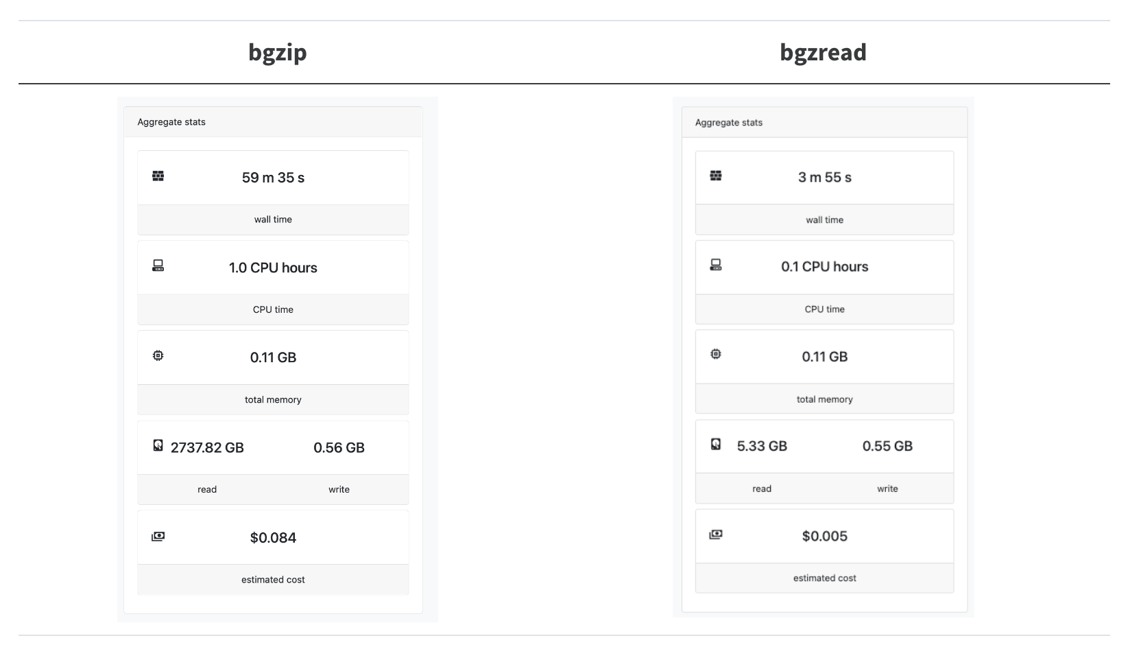
Astonishingly, this results in a 14.8x speedup, and we are reading 240x less data!
The bgzip+bash loop is not quite so bad as it looks here since in production, we can actually split up the 20k sequences into chunks of around 500-1k sequences and batch-process them. However, it is clearly preferable not to have to set up a single bgzip CLI call for every seek + read/deflate operation we need to do.

Understanding GZI Files

Under the hood, BGZF uses another file to track the position of the independently-compressed GZip blocks, called the gzip-index or GZI file. This file uses the .gzi extension. It consists of the compressed and uncompressed offsets of the blocks, as 64-bit unsigned integers – and starting with the second block of course, the first block will always start at (0, 0). But don’t bother trying to read this file directly, fellow human, it’s in a binary format.

Earlier in this post, I made the claim that part of what we gain by using noodles is not just that Rust loops are faster than BASH loops, but that by writing our own program, we only have to read the GZI file once. Our script gets the GZip block positions, and then we can look up our sequences iteratively within those blocks. In bgzip, we have to read in the GZI file independently every time we want to read a position.

Let’s take a look at how long each program is spending reading this file. We can do this using strace, a tool available in Linux. Since both bgzip’s C routines and Rust’s noodles library are at the end of the day using the system calls to read files, strace can tell us when those calls are happening.

For strace, we’ll alias a command that asks traces of openat, reads and close file operations and the flags -ttt will give us timestamps. Finally, we’ll pipe the log (which would normally go into stdout) into a file:

$ alias stracet="strace -ttt -o >(cat >strace.log) -e trace=openat,close,read"

Now let’s call this command for a single bgzip run, for an arbitrary sequence and parse the log file to see where the gzi is getting open and read:

$ stracet bgzip -b 112093709 -s 1149 ca29_soil2_aa_sub.fasta.gz > seq.fa
$ sed -rn '/openat\(.*\.gzi\"/,/close/p' strace.log
1677366815.387446 openat(AT_FDCWD, "ca29_soil2_aa_sub.fasta.gz.gzi", O_RDONLY) = 5
1677366815.388736 read(5, "n\23\0\0\0\0\0\0$\221\0\0\0\0\0\0\0\377\0\0\0\0\0\0^\"\1\0\0\0\0\0"..., 4096) = 4096
1677366815.389304 read(5, "\0\0\377\0\0\0\0\0\311\2\220\0\0\0\0\0\0\377\377\0\0\0\0\0\7\221\220\0\0\0\0\0"..., 4096) = 4096
1677366815.389667 read(5, "\0\0\376\1\0\0\0\0h\215\37\1\0\0\0\0\0\377\376\1\0\0\0\0\370\34 \1\0\0\0\0"..., 4096) = 4096
1677366815.389938 read(5, "\0\0\375\2\0\0\0\0\201$\257\1\0\0\0\0\0\377\375\2\0\0\0\0\233\266\257\1\0\0\0\0"..., 4096) = 4096
1677366815.390206 read(5, "\0\0\374\3\0\0\0\0c\233>\2\0\0\0\0\0\377\374\3\0\0\0\0\27*?\2\0\0\0\0"..., 4096) = 4096
1677366815.390468 read(5, "\0\0\373\4\0\0\0\0/\331\315\2\0\0\0\0\0\377\373\4\0\0\0\0>g\316\2\0\0\0\0"..., 4096) = 4096
1677366815.390690 read(5, "\0\0\372\5\0\0\0\0hZ]\3\0\0\0\0\0\377\372\5\0\0\0\0Z\351]\3\0\0\0\0"..., 4096) = 4096
1677366815.391017 read(5, "\0\0\371\6\0\0\0\0y\376\354\3\0\0\0\0\0\377\371\6\0\0\0\0U\216\355\3\0\0\0\0"..., 4096) = 4096
1677366815.391344 read(5, "\0\0\370\7\0\0\0\0\236\230|\4\0\0\0\0\0\377\370\7\0\0\0\0\270*}\4\0\0\0\0"..., 4096) = 4096
1677366815.391668 read(5, "\0\0\367\10\0\0\0\0\311\34\f\5\0\0\0\0\0\377\367\10\0\0\0\0\335\254\f\5\0\0\0\0"..., 4096) = 4096
1677366815.391938 read(5, "\0\0\366\t\0\0\0\0\206\217\233\5\0\0\0\0\0\377\366\t\0\0\0\0\347\35\234\5\0\0\0\0"..., 4096) = 4096
1677366815.392226 read(5, "\0\0\365\n\0\0\0\0\212\16+\6\0\0\0\0\0\377\365\n\0\0\0\0A\237+\6\0\0\0\0"..., 4096) = 4096
1677366815.392492 read(5, "\0\0\364\v\0\0\0\0r\246\272\6\0\0\0\0\0\377\364\v\0\0\0\0'6\273\6\0\0\0\0"..., 4096) = 4096
1677366815.392724 read(5, "\0\0\363\f\0\0\0\0\276\37J\7\0\0\0\0\0\377\363\f\0\0\0\0\217\257J\7\0\0\0\0"..., 4096) = 4096
1677366815.393001 read(5, "\0\0\362\r\0\0\0\0z\231\331\7\0\0\0\0\0\377\362\r\0\0\0\0\f,\332\7\0\0\0\0"..., 4096) = 4096
1677366815.393291 read(5, "\0\0\361\16\0\0\0\0\270\\i\10\0\0\0\0\0\377\361\16\0\0\0\0\355\354i\10\0\0\0\0"..., 4096) = 4096
1677366815.393542 read(5, "\0\0\360\17\0\0\0\0.\311\370\10\0\0\0\0\0\377\360\17\0\0\0\0\226V\371\10\0\0\0\0"..., 4096) = 4096
1677366815.393788 read(5, "\0\0\357\20\0\0\0\0\210g\210\t\0\0\0\0\0\377\357\20\0\0\0\0\330\370\210\t\0\0\0\0"..., 4096) = 4096
1677366815.394110 read(5, "\0\0\356\21\0\0\0\0\f\342\27\n\0\0\0\0\0\377\356\21\0\0\0\0\23t\30\n\0\0\0\0"..., 4096) = 4096
1677366815.394317 read(5, "\0\0\355\22\0\0\0\0~u\247\n\0\0\0\0\0\377\355\22\0\0\0\0d\4\250\n\0\0\0\0"..., 4096) = 1768
1677366815.394678 close(5)              = 0

We can see the gzi file being open, and the bytes being read into the bgzip program’s buffer and finally closed. Each operation is preceded by a UTC timestamp that we can use to calculate the how much time (in seconds) the program is operating on the file:

$ gzitime () {
   timestamps=( `sed -rn '/openat\(.*\.gzi\"/,/close/p' $1 |
    awk -v ORS=" " 'NR == 1 { print $1; } END { print $1; }'` )
   bc <<< "${timestamps[1]} - ${timestamps[0]}"
}

A short explanation of the above bash function: we’re opening the log file and finding all the lines between opening and closing the gzi file, as before. Then, we’re using awk to grab the first and last timestamps to calculate the time between those operations (which is all the file reads) via the basic calculator (bc) shell command.

$ gzitime strace.log
.007232

7.2 milliseconds doesn’t seem like a lot, but do that again and again, over 3000 independent runs, and it explains what our bash-looped bgzip program is spending over half of its time doing.

Compare this to our Rust program:

$ stracet bgzread ca29_soil2_aa_sub.fasta.gz <( echo "112093709 1149" ) > seq.fa
$ gzitime strace.log
.004572

Not only does this read the index a bit faster than bgzip; it also only runs once!

Indexing the Locations of Sequences in Compressed fasta Files

Clearly, we have already got some significant and actionable performance gains by implementing our own tool in Rust. This is useful, but it turns out that generating the location file for the header positions in the block GZipped-formatted fasta file is actually an even bigger bottleneck than reading locations.

Could we also turn that python script into a Rust command line tool?

I won’t show the whole program (so please don’t try to compile this at home!) but here is a snippet to give you a flavor:

// bgzindex snippet
while let Ok(num) = reader.read_line(&mut line) {

 // Supressed code: updating block_i //
 // Get current block offset from global index //
 block_offset = bgzf_index[block_i];

 if line.starts_with('>') {
   if size > 0 {
       // Write the size of the previously found record
       write_size(&mut writer, size);
   }
   // We found a new record so reset size counter
   size = 0;

   // Write the current record name
   let name: &str = &line.to_string();
   write_name(&mut writer, &name[1..(num-1)]); //subset to trim out < & newline

   // Write the current position
   let virtual_pos = block_offset + (reader.virtual_position().uncompressed() as u64) - (num as u64);
   write_pos(&mut writer, virtual_pos);
 }

 size += num;
 line.clear(); // Clear the line buffer for the next line
}

In this program, we need to keep track of three pieces of data: the sequence name (from the fasta header); the start position of the uncompressed sequence record (pos – position); and size (the number of uncompressed bytes following the start position). We have three convenience functions that I’m not showing the bodies of — write_name, write_pos and write_size — but these simply handle writing the output in the correct three column format.

To summarize the program, whenever we encounter a line that starts with a < character we know we’ve hit a new record. So, we’ll write out the size of the previous record, if one exists yet. Then, we’ll write out the new name – the whole header line except the start token and the final newline. The size (the number of uncompressed characters) of the final sequence record is also easy – we just need to keep a running sum of the size of all the lines associated with that sequence record.

Now the tricky part: we need to calculate the start position. In the python version of this code, we uncompressed the entire file first, so we could just use one global, position tracker. However in the Rust implementation, we want to take advantage of the block format. So, we’ll use the BGZip index (stored in the gzi file) to calculate a global offset relative to the virtual_position of the reader within the block and the start of the block_offset. We’ll just need to keep track of which block we’re in — that’s the block_i indexing variable — and use a local copy of bgzf_index, which is just a vector containing the uncompressed block start positions, which is read directly from the gzi file.

Finally, since reader.read_line function puts our cursor at the end of the line, we need to subtract the line length, num, to get the start position.

Let’s see how this program does:

$ time bgzindex ca29_soil2_aa_sub.fasta.gz ca29_soil2_aa_sub.fasta.loc
real    0m14.650s
user    0m2.745s
sys 0m1.328s

Which is a very nice speedup over the Python script (which took over a minute).

We can even try to parallelize the indexing over multiple threads:

$ time bgzindex ca29_soil2_aa_sub.fasta.gz ca29_soil2_aa_sub.fasta.loc 2
real    0m12.395s
user    0m2.976s
sys 0m0.966s

That’s a 6x speedup all told! Additional cores don’t seem to help much beyond two, however.

And of course the location file looks the same as before:

$ head -n 2 ca29_soil2_aa_sub.fasta.loc && echo "..." && tail -n 2 ca29_soil2_aa_sub.fasta.loc
ca29_soil2_c51cf9d4-216c-4963-8f9b-65ee6b197a07_1   0   116
ca29_soil2_c51cf9d4-216c-4963-8f9b-65ee6b197a07_4   116 448
...
ca29_soil2_99a091d5-f352-4e66-8a50-3c48d2070870_19  324714018   187
ca29_soil2_e966a3b0-d674-47bb-b8b4-6db071c3e3f4_5   324714205   456

Our new bgzindex has some details that lets it take advantage of multithreading. Primarily, we are using the gzi (block gzipped index) file to keep track of the reader’s current virtual position relative to the current block. This adds a bit of overhead at first (we need to read and store the data in the block indexes) but it means that we will always know our global position from within the block we are reading from.

This is important because:

  • We can ditch the global position tracker needed in the Python version of the script, which frees us up to do multithreaded gzip block decompression.
  • Therefore, we avoid annoying the Rust borrow checker by trying to do something like change the value of the reader after it has been “moved” (e.g. read into the buffer).

Let’s try this out on a real-word hard case, indexing the locations of the amino acid sequences in the entire ca29 library.

Nextflow pipeline screenshot of indexing

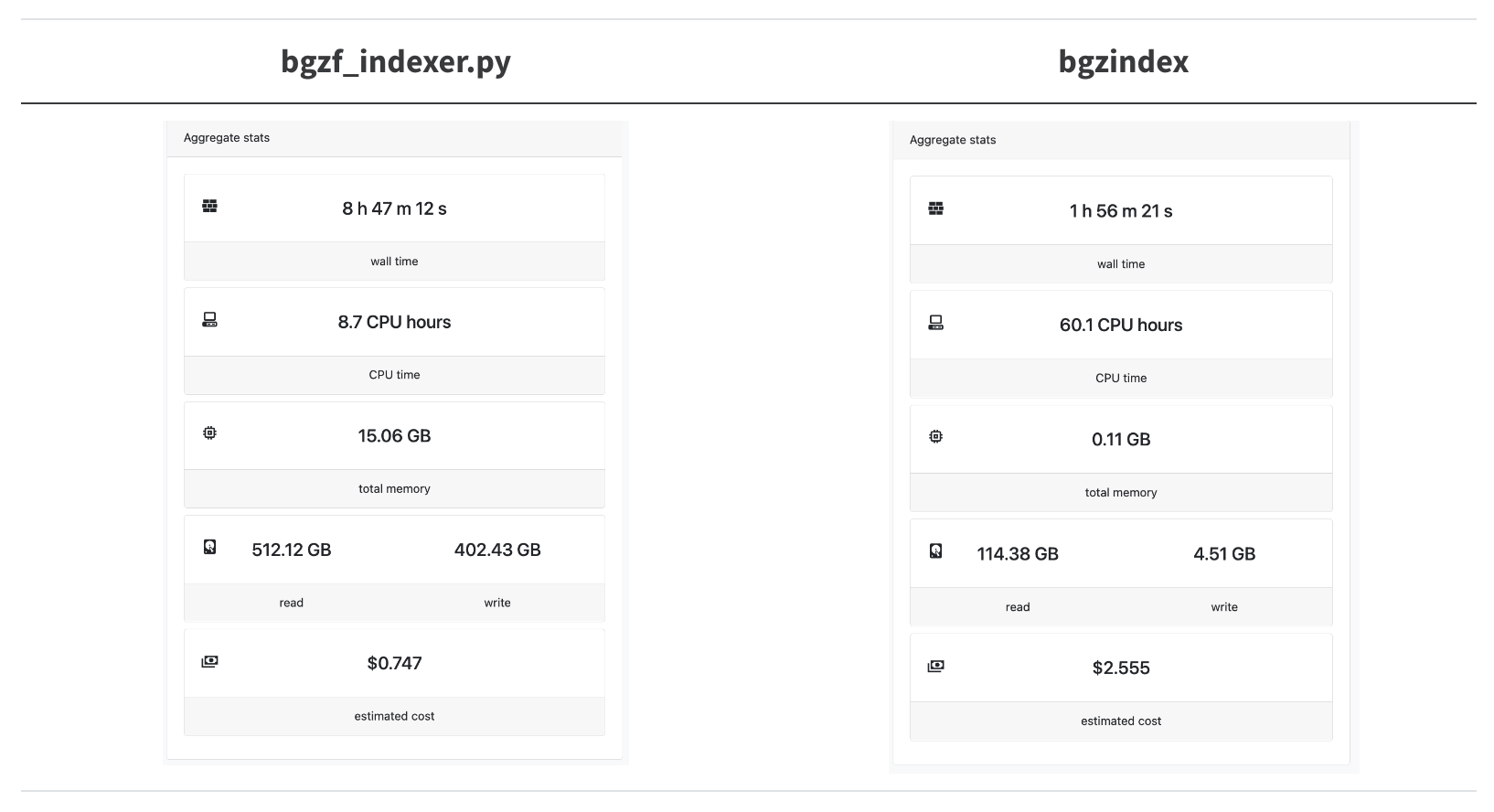
A 4.5x speedup! We’re trying to parallelize as much as possible so we overshot the mark for how many CPUs bgzindex needs (and we overpaid for an instance in this case).

Concluding Remarks

Overall, I’ve been impressed at how easy it has been for me to get up running on Rust. Thanks to reliable, community-supported packages like noodles, I’ve been writing high-performing code after just a few months of learning the basics from “the book”.

I’ve been able to write code that is easy to read, simple to package up and distribute, and has allowed us to crunch through our massive datasets even faster and more reliably.

(Feature photo by Joshua Sortino on Unsplash)

Rapid Data Retrieval from Very Large Files

Background

A core challenge for bioinformatics in metagenomics is that many standard bioinformatics tools are not built to handle datasets of the size of our metagenomic libraries. At the same time, the continued rapid evolution of the field and development of new methods requires that we maintain compatibility with the standard bioinformatic working environment – in other words, if we want to keep up with the state of the field, we must be able to provide command-line access to standard file types (FASTA, GFF, GBK, etc) generated from our data. We also need to be able to subset our data quickly and easily. For example, while we may need or want to operate on the whole library when performing homology searches, once we’ve completed that search, we’ll often want to work with just a subset of the search results for further analysis. In other words, we need: our entire library accessible in a commonly acceptable format, the ability to rapidly subset our data for additional downstream processing, and we need this full set of capabilities available within something that looks like a standard Linux command-line environment. Finally, experience has shown that the closer we can hew to using standard Linux-based tools, the easier it is for our scientists and bioinformaticians to work with our data, the lower the support burden, and the faster we can iterate on methods.

Plainly stated, we need a fast and easy way to store and extract subsets of data from extremely large text files. Let’s investigate some options.

Tools

We’ll be relying on the time command to give us the time a program takes to run, top for memory, and pv to provide us the speed at which a file is being read. time and top are standard Linux tools, and pv is available via the pv package in most distributions.

Setup

The specific problem we’re tackling today is providing fast access and retrieval of gene annotations from a GFF file covering an entire metagenomic library. The GFF format was chosen because it’s simple, supports multiple sequences in one file, allows us to store and retrieve just the gene annotations, is widely supported by standard tooling, and can be converted into other formats as needed.

The CA29 Library

We’ll be working with one library for the duration of this post – the CA29 soil bacterial library. We’ve chosen this one because it’s one of our largest libraries – if we’ve got a solution that works for CA29, we’ve got a solution that works for everything. If you’d like more information about our libraries, our recent paper Precision Discovery of Novel Inhibitors of Cancer Target HsMetAP1 from Vast Metagenomic Diversity includes details on their construction and use.

Some quick stats on the library, for reference:

  • Sequences: ~150M
  • Annotations: ~1.6B
  • Uncompressed Size: 235Gb
  • Compressed Size: 24Gb

Note that depending on the context below I may use either GiB or Gb, depending on what the tool I’m using puts out. In both cases, the term refers to 2^30, or 1024^3, bytes.

Goals

Our goal here is to be able to easily retrieve the gene calls for an individual sequence from our combined library. We’d like to do this quickly enough for it to be practical as part of other pipelines, which we’ll define as “less than a minutes to retrieve the GFF for a sequence,” and we’d also like to keep the computational resources down to an arbitrarily-chosen limit of 2 CPUs and 4Gb of memory, as this will fit inside almost any process we run and stands a very low probability of bankrupting the company.

Approaches

Tabix

The standard tool for retrieval of subsets of data from GFF files is tabix, which is part of the htslib package. Tabix works by creating an index file that maps sequence IDs to their positions in the compressed GFF file, and then using this index to provide rapid lookup and retrieval by sequence ID or sequence ID and location. Tabix, however, suffers from two major limitations for our use case – first, as of the latest version, Tabix has a bug which causes it to crash if the total length of all of the sequence IDs in the GFF file it is indexing exceeds 2^31 bytes. We use UUIDs for sequence names, and so this imposes a limit of around 50 million sequences, which is on the low side for one of our libraries. Second, Tabix’s memory use is extremely high for large datasets – when searching a 12Gb compressed GFF file, Tabix requires 32Gb of memory.

Not all’s lost, though. Under the hood, Tabix uses another utility, BGZip, to facilitate its quick retrieval. BGZip turns out to be a real gem, both in its use and construction.

BGZip

BGZip makes use of a quirk in the widely-used and supported gzip file format – that you can concatenate multiple gzipped files together and the result is still a valid gzip archive. BGZip takes this to an extreme – when compressing a file, it splits the file into small chunks, gzips them independently, and then generates an index file mapping locations from the uncompressed file into the compressed file.

[            long_file.gff             ]
                  ↓
[ part 1 ][ part 2 ][ part 3 ][ part 4 ]
        ↓ Compressed and Indexed ↓
[a][b][c][d] + { part 1: a; part 2: b; ...}

This gives BGZip two neat tricks. One, which we’ll get back to later, is that it can compress and decompress multiple chunks at a time, since each chunk is fixed size and independent of its surroundings. The second is that it can retrieve subsections of the compressed file almost instantly:

# Relative size of the gzipped and uncompressed files:
$ ls -alh
total 259G
drwxrwxr-x 2 ubuntu ubuntu 4.0K Oct  4 21:31 .
drwxr-xr-x 9 ubuntu root   4.0K Oct  4 21:25 ..
-rw-rw-r-- 1 ubuntu ubuntu 235G Oct  4 21:35 ca29.gff
-rwxr-xr-x 1 ubuntu ubuntu  24G Oct  4 21:29 ca29.gff.gz
-rwxr-xr-x 1 ubuntu ubuntu  59M Oct  4 21:29 ca29.gff.gz.gzi

# ('.gzi' is bgzip's index - note it's only 60M for our 24Gb file)

# Retrieving a specific section of the uncompressed file, using `tail` and `head`:

$ time tail -c +251262670684 ca29.gff | head -c 60
##sequence-region fffff5f2-0bcb-4560-8399-c86c632969b8 1 125
real	0m0.001s
user	0m0.002s
sys	0m0.000s

# Retrieving a specific section of the compressed file using bgzip - note
# the start and size are the same as the uncompressed reads above:

$ time bgzip -b 251262670684 -s 60 ca29.gff.gz
#sequence-region fffff5f2-0bcb-4560-8399-c86c632969b8 1 1257
real	0m0.054s
user	0m0.025s
sys	0m0.029s

# Retrieval time does not scale with the size of the chunk retrieved:

$ time bgzip -b 251262670683 -s 62000000 ca29.gff.gz > /dev/null

real	0m0.054s
user	0m0.019s
sys	0m0.035s

So we’ve got the first part of our solution – nearly instantaneous retrieval of a subset of an excessively large gzipped file based on start location and size. By adding a sequence location index next to our GFF file with the sequence ID, start location, and size of the associated entries, we can get almost instant sequence retrieval:

# Our location index file:

$ head ca29.gff.loc.tsv
seq_id	offset	length
00000020-3ae5-4305-8de8-1bfceaa81f1c	16	1276
00000035-1d98-4718-960c-e1c0f9fda8c9	1292	937
00000057-0ac5-467f-a37f-3e64cf9928e8	2229	937
0000005c-da49-428c-95e5-342515731bc0	3166	937
00000076-c423-45c5-86b1-52fed94afbbf	4103	937
0000008a-7735-43f7-95fa-64ab84372ca1	5040	1617
000000f9-d5ca-4723-876d-b9942873d8cb	6657	602
0000015b-02d1-4c22-8b2f-8e723961f5fb	7259	939
00000197-45d6-4d40-8ab6-102b3e0000e8	8198	937

# Grab a random sequence from the end:

$ tail -n50 ca29.gff.loc.tsv | head -n1
fffffb2f-878d-4b23-a82f-573fbc1fad5f	251262762041	935

# Retrieve the gene calls from the compressed GFF:

$ time bgzip -b 251262762041 -s 935 ca29.gff.gz
##sequence-region fffffb2f-878d-4b23-a82f-573fbc1fad5f 1 1093
fffffb2f-878d-4b23-a82f-573fbc1fad5f	annotation	remark	1	1093	.	.	.	molecule_type=DNA;topology=linear
fffffb2f-878d-4b23-a82f-573fbc1fad5f	feature	region	1	1093	.	.	.	ID=fffffb2f-878d-4b23-a82f-573fbc1fad5f
fffffb2f-878d-4b23-a82f-573fbc1fad5f	feature	CDS	1	87	.	-	0	ID=fffffb2f-878d-4b23-a82f-573fbc1fad5f_1;gene_id=fffffb2f-878d-4b23-a82f-573fbc1fad5f_1;gene_number=1;name=fffffb2f-878d-4b23-a82f-573fbc1fad5f_1
fffffb2f-878d-4b23-a82f-573fbc1fad5f	feature	exon	1	87	.	-	.	gene_id=fffffb2f-878d-4b23-a82f-573fbc1fad5f_1;gene_number=1
fffffb2f-878d-4b23-a82f-573fbc1fad5f	feature	CDS	212	1093	.	-	0	ID=fffffb2f-878d-4b23-a82f-573fbc1fad5f_2;gene_id=fffffb2f-878d-4b23-a82f-573fbc1fad5f_2;gene_number=2;name=fffffb2f-878d-4b23-a82f-573fbc1fad5f_2
fffffb2f-878d-4b23-a82f-573fbc1fad5f	feature	exon	212	1093	.	-	.	gene_id=fffffb2f-878d-4b23-a82f-573fbc1fad5f_2;gene_number=2

real	0m0.059s
user	0m0.029s
sys	0m0.025s

Using grep, we can retrieve the locations for an individual sequence id:

$ grep fffffb2f-878d-4b23-a82f-573fbc1fad5f ca29.gff.loc.tsv
fffffb2f-878d-4b23-a82f-573fbc1fad5f	251262762041	935

$ bgzip -b 251262762041 -s 935 ca29.gff.gz
##sequence-region fffffb2f-878d-4b23-a82f-573fbc1fad5f 1 1093
fffffb2f-878d-4b23-a82f-573fbc1fad5f	annotation	remark	1	1093	.	.	.	molecule_type=DNA;topology=linear
fffffb2f-878d-4b23-a82f-573fbc1fad5f	feature	region	1	1093	.	.	.	ID=fffffb2f-878d-4b23-a82f-573fbc1fad5f
fffffb2f-878d-4b23-a82f-573fbc1fad5f	feature	CDS	1	87	.	-	0	ID=fffffb2f-878d-4b23-a82f-573fbc1fad5f_1;gene_id=fffffb2f-878d-4b23-a82f-573fbc1fad5f_1;gene_number=1;name=fffffb2f-878d-4b23-a82f-573fbc1fad5f_1
fffffb2f-878d-4b23-a82f-573fbc1fad5f	feature	exon	1	87	.	-	.	gene_id=fffffb2f-878d-4b23-a82f-573fbc1fad5f_1;gene_number=1
fffffb2f-878d-4b23-a82f-573fbc1fad5f	feature	CDS	212	1093	.	-	0	ID=fffffb2f-878d-4b23-a82f-573fbc1fad5f_2;gene_id=fffffb2f-878d-4b23-a82f-573fbc1fad5f_2;gene_number=2;name=fffffb2f-878d-4b23-a82f-573fbc1fad5f_2
fffffb2f-878d-4b23-a82f-573fbc1fad5f	feature	exon	212	1093	.	-	.	gene_id=fffffb2f-878d-4b23-a82f-573fbc1fad5f_2;gene_number=2

We can even do this as a one-liner, if we’re clever:

# Isn't bash grand?
$ bgzip $( grep fffffb2f-878d-4b23-a82f-573fbc1fad5f ca29.gff.loc.tsv | awk '{ print "-b", $2, "-s", $3 }' ) ca29.gff.gz
##sequence-region fffffb2f-878d-4b23-a82f-573fbc1fad5f 1 1093
fffffb2f-878d-4b23-a82f-573fbc1fad5f	annotation	remark	1	1093	.	.	.	molecule_type=DNA;topology=linear
fffffb2f-878d-4b23-a82f-573fbc1fad5f	feature	region	1	1093	.	.	.	ID=fffffb2f-878d-4b23-a82f-573fbc1fad5f
fffffb2f-878d-4b23-a82f-573fbc1fad5f	feature	CDS	1	87	.	-	0	ID=fffffb2f-878d-4b23-a82f-573fbc1fad5f_1;gene_id=fffffb2f-878d-4b23-a82f-573fbc1fad5f_1;gene_number=1;name=fffffb2f-878d-4b23-a82f-573fbc1fad5f_1
fffffb2f-878d-4b23-a82f-573fbc1fad5f	feature	exon	1	87	.	-	.	gene_id=fffffb2f-878d-4b23-a82f-573fbc1fad5f_1;gene_number=1
fffffb2f-878d-4b23-a82f-573fbc1fad5f	feature	CDS	212	1093	.	-	0	ID=fffffb2f-878d-4b23-a82f-573fbc1fad5f_2;gene_id=fffffb2f-878d-4b23-a82f-573fbc1fad5f_2;gene_number=2;name=fffffb2f-878d-4b23-a82f-573fbc1fad5f_2
fffffb2f-878d-4b23-a82f-573fbc1fad5f	feature	exon	212	1093	.	-	.	gene_id=fffffb2f-878d-4b23-a82f-573fbc1fad5f_2;gene_number=2

So, knowing nothing except the sequence ID we want to find and the library it’s in, we can quickly and efficiently grab all the gene calls for that sequence ID as a GFF file.

But, there’s a catch – our location file is Big! It contains one line for every sequence in the GFF file:

$ ls -alh ca29.gff.loc.tsv
-rw-rw-r-- 1 ubuntu ubuntu 7.8G Oct  4 22:02 ca29.gff.loc.tsv

So let’s dig into some options for dealing with this file.

Compressing the Index File

We now have an index file formatted as follows:

seq_id  offset  length
00000020-3ae5-4305-8de8-1bfceaa81f1c    16  1276
00000035-1d98-4718-960c-e1c0f9fda8c9    1292    937

Note this file is extremely dense – we have the sequence ID, offset, and length, and very little else. Consequently, the file doesn’t compress particularly well:

# Uncompressed:
$ du -hs ca29.gff.loc.tsv
7.8G	ca29.gff.loc.tsv

# Compressed:
$ du -hs ca29.gff.loc.tsv.gz
3.7G	ca29.gff.loc.tsv.gz

There’s just not a lot of slack to take out here. We could do something similar to BGZip and use a binary format, as opposed to just a standard ASCII file, and we might get some savings there, but then we’d need to build and distribute a toolchain for dealing with our proprietary index format, so that’s off the table for now.
Note also that the uncompressed index is comparable to the compressed GFF itself – 8Gb vs 24Gb, or about a third the size. We’d prefer to keep the compressed version. However, we quickly hit a problem: finding individual sequences from the gzipped file is a whole lot slower than the raw text format:

# Uncompressed:
$ time cat ca29.gff.loc.tsv | grep fffffb2f-878d-4b23-a82f-573fbc1fad5f
fffffb2f-878d-4b23-a82f-573fbc1fad5f	251262762041	935

real	0m4.004s
user	0m2.328s
sys	0m4.776s

# Compressed:
$ time zcat ca29.gff.loc.tsv.gz | grep fffffb2f-878d-4b23-a82f-573fbc1fad5f
fffffb2f-878d-4b23-a82f-573fbc1fad5f	251262762041	935

real	1m0.754s
user	1m0.947s
sys	0m5.050s

Yowza! A minute to look up a single sequence in our compressed location file? What’s going on?
Let’s pull out pv and see where our bottleneck is. pv is a lovely little tool that works roughly like cat, but will show how fast it’s passing data along. Linux pipes affect our speed, so we’ll throw cat in between pv and grep just to make things fair:

# Uncompressed:
$ time pv ca29.gff.loc.tsv | cat - | grep fffffb2f-878d-4b23-a82f-573fbc1fad5f
7.73GiB 0:00:03 [1.95GiB/s] [==========================================>] 100%
fffffb2f-878d-4b23-a82f-573fbc1fad5f	251262762041	935

real	0m3.745s
user	0m2.486s
sys	0m2.580s

# Compressed
$ time pv ca29.gff.loc.tsv.gz | zcat - | grep fffffb2f-878d-4b23-a82f-573fbc1fad5f
3.62GiB 0:01:01 [60.3MiB/s] [==========================================>] 100%
fffffb2f-878d-4b23-a82f-573fbc1fad5f	251262762041	935

real	1m1.473s
user	1m1.319s
sys	0m5.835s

Decompressing our compressed archive slows us down from nearly 2GiB/s to a piddling 60MiB/s. Our gzipped location file is half the size, but takes 30x as long to retrieve sequences from. That’s not great. The difference reduces a bit if we decide to search for multiple sequence IDs:

# 10 sequence IDs to search for
$ cat seq_ids.txt
fef21bda-479c-445b-affd-d04761795174
fdd86a15-1848-4a2b-be05-f9d62a0ee538
fcdd2245-17b1-4a7a-9f67-1a34802aefd3
ffc97fde-cf41-4440-b50b-86abad46f415
ff9fa0a4-7042-45bc-bf70-c502a1e49522
feed9c3a-9831-4c42-81a9-d072f728c9f2
fce7cd9b-8cf9-41f7-a4a2-04a7814e41b6
fd7fae42-f746-4934-b71e-d738d8da31bc
fd55e51f-6773-4eb4-871d-4174e99547a9
fd581f3d-6ce0-4895-8b38-083c091a4729

# Uncompressed:
$ time pv ca29.gff.loc.tsv | cat - | grep --file seq_ids.txt
fcdd2245-17b1-4a7a-9f67-1a34802aefd3	248192112609	943
fce7cd9b-8cf9-41f7-a4a2-04a7814e41b6	248232660866	597
fd55e51f-6773-4eb4-871d-4174e99547a9	248655071744	597
fd581f3d-6ce0-4895-8b38-083c091a4729	248663484363	1276
fd7fae42-f746-4934-b71e-d738d8da31bc	248815519201	2291
fdd86a15-1848-4a2b-be05-f9d62a0ee538	249153912987	937
feed9c3a-9831-4c42-81a9-d072f728c9f2	250214540699	597
fef21bda-479c-445b-affd-d04761795174	250231619577	599
ff9fa0a4-7042-45bc-bf70-c502a1e49522	250893965638	941
ffc97fde-cf41-4440-b50b-86abad46f415	251054447078	937
7.73GiB 0:00:10 [ 781MiB/s] [==========================================>] 100%

real	0m10.132s
user	0m8.352s
sys	0m6.810s

# Compressed:
$ time pv ca29.gff.loc.tsv.gz | zcat - | grep --file seq_ids.txt > /dev/null
3.62GiB 0:01:02 [58.8MiB/s] [==========================================>] 100%

real	1m2.997s
user	1m8.761s
sys	0m5.691s

Not a big difference for our compressed reads – that’s obviously bottlenecked on decompression – but our uncompressed reads drop to around 800MiB/s, and it takes about 10s to get our results. This is probably as fast as we’re going to get with the index file approach, so let’s keep this as a benchmark.

First, though, let’s try a very different approach.

Using Sqlite3

What if we went with a database instead? Sqlite works fine as a command line utility, and it should certainly be faster than grepping through a text file – and indeed it is:

# The SQLite DB:
$ sqlite3 ca29.gff.sqlite3
SQLite version 3.38.2 2022-03-26 13:51:10
Enter ".help" for usage hints.
sqlite> .schema
CREATE TABLE location (
contig_id TEXT PRIMARY KEY,
start INTEGER NOT NULL,
length INTEGER NOT NULL
);
sqlite> select * from location limit 5;
seq_id|offset|length
00000020-3ae5-4305-8de8-1bfceaa81f1c|16|1276
00000035-1d98-4718-960c-e1c0f9fda8c9|1292|937
00000057-0ac5-467f-a37f-3e64cf9928e8|2229|937
0000005c-da49-428c-95e5-342515731bc0|3166|937
sqlite>

# Single sequence retrieval is almost instantaneous
$ time sqlite3 -tabs ca29.gff.sqlite3 'select * from location where contig_id = "fef21bda-479c-445b-affd-d04761795174"'
fef21bda-479c-445b-affd-d04761795174	250231619577	599

real	0m0.002s
user	0m0.002s
sys	0m0.000s

# Multiple sequence retrieval takes about the same time
$ time sqlite3 -tabs ca29.gff.sqlite3 "select * from location where contig_id in ('fef21bda-479c-445b-affd-d04761795174','fdd86a15-1848-4a2b-be05-f9d62a0ee538','fcdd2245-17b1-4a7a-9f67-1a34802aefd3','ffc97fde-cf41-4440-b50b-86abad46f415','ff9fa0a4-7042-45bc-bf70-c502a1e49522','feed9c3a-9831-4c42-81a9-d072f728c9f2','fce7cd9b-8cf9-41f7-a4a2-04a7814e41b6','fd7fae42-f746-4934-b71e-d738d8da31bc','fd55e51f-6773-4eb4-871d-4174e99547a9','fd581f3d-6ce0-4895-8b38-083c091a4729')"
fcdd2245-17b1-4a7a-9f67-1a34802aefd3	248192112609	943
fce7cd9b-8cf9-41f7-a4a2-04a7814e41b6	248232660866	597
fd55e51f-6773-4eb4-871d-4174e99547a9	248655071744	597
fd581f3d-6ce0-4895-8b38-083c091a4729	248663484363	1276
fd7fae42-f746-4934-b71e-d738d8da31bc	248815519201	2291
fdd86a15-1848-4a2b-be05-f9d62a0ee538	249153912987	937
feed9c3a-9831-4c42-81a9-d072f728c9f2	250214540699	597
fef21bda-479c-445b-affd-d04761795174	250231619577	599
ff9fa0a4-7042-45bc-bf70-c502a1e49522	250893965638	941
ffc97fde-cf41-4440-b50b-86abad46f415	251054447078	937

real	0m0.002s
user	0m0.002s
sys	0m0.000s

Great! The SQLite3 database lookup is almost immediate! So what’s the problem? Well:

$ du -hs ca29.gff.sqlite3
16G	ca29.gff.sqlite3

The problem is the database is on the order of 2/3rds the size of the compressed file it’s searching. This might be a fine trade-off in some cases – after all, it’s providing nearly instantaneous lookups, which might be worth the storage space:

$ time bgzip $( sqlite3 -tabs ca29.gff.sqlite3 'select * from location where contig_id = "fffffb2f-878d-4b23-a82f-573fbc1fad5f"' | awk '{ print "-b", $2, "-s", $3 }' ) ca29.gff.gz
##sequence-region fffffb2f-878d-4b23-a82f-573fbc1fad5f 1 1093
fffffb2f-878d-4b23-a82f-573fbc1fad5f	annotation	remark	1	1093	.	.	.	molecule_type=DNA;topology=linear
fffffb2f-878d-4b23-a82f-573fbc1fad5f	feature	region	1	1093	.	.	.	ID=fffffb2f-878d-4b23-a82f-573fbc1fad5f
fffffb2f-878d-4b23-a82f-573fbc1fad5f	feature	CDS	1	87	.	-	0	ID=fffffb2f-878d-4b23-a82f-573fbc1fad5f_1;gene_id=fffffb2f-878d-4b23-a82f-573fbc1fad5f_1;gene_number=1;name=fffffb2f-878d-4b23-a82f-573fbc1fad5f_1
fffffb2f-878d-4b23-a82f-573fbc1fad5f	feature	exon	1	87	.	-	.	gene_id=fffffb2f-878d-4b23-a82f-573fbc1fad5f_1;gene_number=1
fffffb2f-878d-4b23-a82f-573fbc1fad5f	feature	CDS	212	1093	.	-	0	ID=fffffb2f-878d-4b23-a82f-573fbc1fad5f_2;gene_id=fffffb2f-878d-4b23-a82f-573fbc1fad5f_2;gene_number=2;name=fffffb2f-878d-4b23-a82f-573fbc1fad5f_2
fffffb2f-878d-4b23-a82f-573fbc1fad5f	feature	exon	212	1093	.	-	.	gene_id=fffffb2f-878d-4b23-a82f-573fbc1fad5f_2;gene_number=2

real	0m0.058s
user	0m0.043s
sys	0m0.017s

But that’s an awful big trade, especially since our previous best of just grep-ing the raw text file for a single result was around 2 seconds. We’re not using this for an inline service, so the difference between 2 seconds and “immediate” really isn’t much for us. Let’s see if we can get any better from our index file.

Back to the Filesystem

So to recap, we’ve got an 8Gb uncompressed TSV file we can compress down to 4Gb, but then we see search times on the order of a minute or so for a set of sequence IDs.

Once again, taking a look at our timings, it’s clear the decompression time is our bottleneck. Taking grep out of the picture entirely makes this really clear:

# No pipes at all, just dump the file as fast as we can
$ time pv ca29.gff.loc.tsv > /dev/null
7.73GiB 0:00:01 [7.61GiB/s] [==========================================>] 100%

real	0m1.017s
user	0m0.016s
sys	0m1.000s

# Pipe to cat - notice we cut our speed roughly in half right
# off the bat if we want to consume our data:
$ time pv ca29.gff.loc.tsv | cat - > /dev/null
7.73GiB 0:00:01 [4.38GiB/s] [==========================================>] 100%

real	0m1.765s
user	0m0.030s
sys	0m2.838s

# Decompressing the gzipped file is what's killing us, though:
$ time pv ca29.gff.loc.tsv.gz | zcat - > /dev/null
3.62GiB 0:00:59 [62.4MiB/s] [==========================================>] 100%

real	0m59.334s
user	0m57.868s
sys	0m1.973s

Let’s add grep back in, just so we’ve got a picture of where we’re trying to get:

# Grep for our set of 10 sequence IDs
$ time pv ca29.gff.loc.tsv | grep --file seq_ids.txt > /dev/null
7.73GiB 0:00:09 [ 832MiB/s] [==========================================>] 100%

real	0m9.511s
user	0m8.164s
sys	0m2.644s

So grep itself is limited to about 800Mb/s for multiple matches.

A Quick Diversion into Alternate Greps

There are a couple alternatives to grep that promise faster searches – let’s take a quick look at ag and ripgrep to see what they offer:

# RipGrep:
$ time pv ca29.gff.loc.tsv | rg --file ./seq_ids.txt  > /dev/null
7.73GiB 0:00:18 [ 422MiB/s] [==========================================>] 100%

real	0m18.735s
user	0m15.821s
sys	0m10.066s

# AG, the "silver searcher" - AG does not support a patterns file:
$ time pv ca29.gff.loc.tsv | ag -F 'fef21bda-479c-445b-affd-d04761795174'
fef21bda-479c-445b-affd-d04761795174	250231619577	599
7.73GiB 0:00:20 [ 380MiB/s] [==========================================>] 100%

real	0m20.781s
user	0m15.630s
sys	0m19.217s

Both tools are half the speed of grep, and ag doesn’t support supplying multiple queries in a file. Generally, both of these tools are built to rapidly search a large tree of files, whereas we’re asking them to search one big file – as always, us humble bioinformaticians are left out in the cold. We’re not going to get saved by a different search utility – it looks like we’re stuck with grep.

Back to BGZip

So our bottleneck is decompression – remember earlier when I mentioned BGZip’s two big tricks? The multi-threaded decompression didn’t matter for us much before, since we were seeking specifically what we needed, but now we’re searching the whole file – let’s see if BGZip’s got something up its sleeve for us. As a reminder, here’s standard zcat:

# Standard zcat:
$ time pv ca29.gff.loc.gz | zcat - > /dev/null
3.61GiB 0:01:03 [58.2MiB/s] [==========================================>] 100%

real	1m3.615s
user	1m2.497s
sys	0m1.620s

And here’s bgzip with no threading, after we recompress the locations file using bgzip:

$ time pv ca29.gff.loc.tsv.gz | bgzip -c -d - > /dev/null
3.62GiB 0:00:24 [ 153MiB/s] [==========================================>] 100%

real	0m24.102s
user	0m22.340s
sys	0m1.819s

Already we’re three times as fast – because BGZip can trade between reading and decompressing and make some better assumptions about the source data, we’re not bottlenecked quite as badly on decompression. But let’s see what happens when we actually use the parallel decompression:

# Two threads
$ time pv ca29.gff.loc.tsv.gz | bgzip --threads 2 -c -d > /dev/null
3.62GiB 0:00:11 [ 320MiB/s] [==========================================>] 100%

real	0m11.573s
user	0m23.952s
sys	0m2.653s

# Four threads:
$ time pv ca29.gff.loc.tsv.gz | bgzip --threads 4 -c -d > /dev/null
3.62GiB 0:00:05 [ 640MiB/s] [==========================================>] 100%

real	0m5.788s
user	0m23.714s
sys	0m2.449s

# Eight threads:
$ time pv ca29.gff.loc.tsv.gz | bgzip --threads 8 -c -d > /dev/null
3.62GiB 0:00:02 [1.23GiB/s] [==========================================>] 100%

real	0m2.953s
user	0m24.297s
sys	0m2.621s

# 16 threads:
$ time pv ca29.gff.loc.tsv.gz | bgzip --threads 16 -c -d > /dev/null
3.62GiB 0:00:02 [1.49GiB/s] [==========================================>] 100%

real	0m2.439s
user	0m29.208s
sys	0m2.514s

These are enormous speedups in decompression, especially compared to the naive zcat approach – BGZip is doing some really fantastic work with threading here. You can see an almost linear increase in read speed right up through 8 threads, although we start to drop off above that – coordination takes its toll, eventually.

Let’s see what this looks like combined with grep. We’ll use 4 threads, and we’ll take pv out of the picture:

$ time bgzip --threads 4 -c -d ca29.gff.loc.tsv.gz | grep --file seq_ids.txt > /dev/null

real	0m10.091s
user	0m33.097s
sys	0m5.670s

10 seconds – that’s roughly what we were getting with the uncompressed search. BGZip’s not as fast as just reading an uncompressed file, but it’s fast enough to keep up with grep – decompression is no longer our bottleneck. BGZip is fast enough that we can keep our compressed index file with no speed sacrifice.

A Couple More Grep Tricks

Two more notes on grep to close out our testing.

First, we’ve been searching for multiple results in our index file, since that’s a relatively normal use case for us, but that actually imposes a pretty steep penalty on grep:

$ time pv ca29.gff.loc.tsv | grep "fef21bda-479c-445b-affd-d04761795174" > /dev/null
7.73GiB 0:00:03 [1.96GiB/s] [==========================================>] 100%

real	0m3.944s
user	0m2.644s
sys	0m2.616s

Fortunately, the real world effects here are pretty limited – BGZip is still fast enough that, roughly, this doesn’t matter:

$ time bgzip --threads 8 -c -d ca29.gff.loc.tsv.gz | grep --file just_one_seq_id.txt > /dev/null

real	0m4.138s
user	0m29.531s
sys	0m5.396s

One change we can make, though, that does make a difference is telling grep when to stop. We’re looking for exactly one line per sequence, so we shouldn’t ever get more lines than we have in our input. The -m flag tells grep how many results to expect:

# Grab a sequence ID towards the front of our file:
$ head -n100 ca29.gff.loc.tsv | tail -n1
00000c54-06f6-438b-9474-c56d4ff130b2	196289	932


# Grep without a hit of our count:
(base) ubuntu@npd-edanielson-work:/data/ca29$ time cat ca29.gff.loc.tsv | grep "00000c54-06f6-438b-9474-c56d4ff130b2" > /dev/null

real	0m3.134s
user	0m0.026s
sys	0m4.138s

# Tell grep how many results to expect:
(base) ubuntu@npd-edanielson-work:/data/ca29$ time cat ca29.gff.loc.tsv | grep -m1 "00000c54-06f6-438b-9474-c56d4ff130b2" > /dev/null

real	0m0.002s
user	0m0.000s
sys	0m0.002s

We’ve been playing a bit of a trick with our timings so far, because we’ve been using the most pathological case we can – 10 sequence IDs all towards the end of the file, which means grep needs to search the entire file to find our results. In more realistic use cases, we’d have a more normally distributed set of sequence IDs, and adding the -m flag to our searches will make a much bigger difference. The takeaway here is that the 10 seconds we saw above could be considered our worst-case scenario – at worst, it will take 10 seconds to retrieve a set of results from our file. We can live with that.

Conclusion

Final Layout

Our final layout for our library includes four files:

  • ca29.gff.gz (24Gb) – The full BGZip-compressed GFF file
  • ca29.gff.gz.gzi (59Mb) – BGZip’s index file
  • ca29.gff.loc.gz (3.7Gb) – The compressed sequence location TSV file
  • ca29.gff.loc.gz.gzi (2.0Mb) – BGZip’s index file

The total space for all four files is around 28Gb, or around 12% the size of our original uncompressed GFF library. Retrieving a single sequence can be performed in one line of bash with only the sequence ID and the library in a matter of seconds:

$ time bgzip $( bgzip -c -d --threads 4 ./ca29.gff.loc.tsv.gz | grep -m1 -F "78ef59ad-94b9-4944-9a3e-e1c171fc0df5" | awk '{ print "-b", $2, "-s", $3 }' ) ca29.gff.gz > 78ef59ad-94b9-4944-9a3e-e1c171fc0df5.gff

real	0m2.803s
user	0m12.415s
sys	0m2.399s

$ cat 78ef59ad-94b9-4944-9a3e-e1c171fc0df5.gff
##sequence-region 78ef59ad-94b9-4944-9a3e-e1c171fc0df5 1 1620
78ef59ad-94b9-4944-9a3e-e1c171fc0df5	annotation	remark	1	1620	.	.	.	molecule_type=DNA;topology=linear
78ef59ad-94b9-4944-9a3e-e1c171fc0df5	feature	region	1	1620	.	.	.	ID=78ef59ad-94b9-4944-9a3e-e1c171fc0df5
78ef59ad-94b9-4944-9a3e-e1c171fc0df5	feature	CDS	2	424	.	-	0	ID=78ef59ad-94b9-4944-9a3e-e1c171fc0df5_1;gene_id=78ef59ad-94b9-4944-9a3e-e1c171fc0df5_1;gene_number=1;name=78ef59ad-94b9-4944-9a3e-e1c171fc0df5_1
78ef59ad-94b9-4944-9a3e-e1c171fc0df5	feature	exon	2	424	.	-	.	gene_id=78ef59ad-94b9-4944-9a3e-e1c171fc0df5_1;gene_number=1
78ef59ad-94b9-4944-9a3e-e1c171fc0df5	feature	CDS	435	1619	.	+	0	ID=78ef59ad-94b9-4944-9a3e-e1c171fc0df5_2;gene_id=78ef59ad-94b9-4944-9a3e-e1c171fc0df5_2;gene_number=2;name=78ef59ad-94b9-4944-9a3e-e1c171fc0df5_2
78ef59ad-94b9-4944-9a3e-e1c171fc0df5	feature	exon	435	1619	.	+	.	gene_id=78ef59ad-94b9-4944-9a3e-e1c171fc0df5_2;gene_number=2

Closing Remarks

Our original goal was to facilitate easy, fast, and cheap extraction of gene calls for a specific sequence from a library-level dataset. BGZip, part of the Samtools/HTSLib package, provides blazing fast indexed access into arbitrarily large gzip-compatible compressed files, with a very small space penalty for its index file. In addition, BGZip’s threaded compression & decompression, as well as some other optimizations, allow us to retrieve specific sequence locations from a compressed text location file as quickly as if the file were not compressed. The combination of these two features give us the ability to retrieve information for one or more sequences from our dataset in a matter of seconds.

Taken together, this allows us to keep our gene calls available on disk in a common bioinformatics format and to work with those files using standard *nix tools. Within our pipelines, we can go from a list of sequence IDs to the gene calls for those individual sequences in seconds. The approach generalizes to other file types as well – any file format in which the data for an individual item is written contiguously in the file and in which a single item can be read individually – such as FASTAs, JSONL, and others – is amenable to this approach.

In our next post, we will explore even faster ways to retrieve data from very large files!

(Feature photo by Joshua Sortino on Unsplash)

Human Interactions in Lab Automation

When you think of lab automation, what comes to mind first? Robots? Rails? Instruments? Data? This is what comes to my mind when I think of automation. Lab Automation has a wide range of topics and applications but also great depths in unexplored opportunities. It can be easy to lose track of why automation is important in a lab.

What would you say if I asked, “What problems should automation solve for a lab?” I talked to numerous experts at Ginkgo, and we all landed on two distinct problem spaces:

  • Humans are spending too much time on tasks that can be automated.
  • Certain tasks are too difficult or impossible for a human to perform.

Sounds simple right? Well, notice how I didn’t talk about walk-away time, reliability, flexibility, or throughput. Let me explain. We often think of walk-away time or throughput as excellent outcomes for our automation tools or ways to measure their success. But the question remains, why? Why is throughput or walk-away time so important to us? For instance, if I were a lab user whose role was to execute experiments in automation but my walk-away time was 100%, what would I be able to achieve with that extra time instead? One can argue reducing the number of users executing tasks is more important than walk-away time. Here is where I think the biggest missed opportunity is. When we think of lab automation, we often think of what a robot is capable of achieving when in reality lab automation should be about humans and how technology can augment human capabilities. It is important to think about automation in terms of what it enables humans to do.

At Ginkgo, we took these problem spaces further. We wanted to come up with essential goals for how we should approach automation, all centered around human interaction. We came up with three.

  • Reduce barriers of entry for humans to leverage automation. This goal is centered around the idea that users of automation shouldn’t be expert programmers or engineers. Tools should be designed for the intended user in the lab and speak its language.
  • Reduce friction for humans to navigate across different levels of automation. This goal is centered around allowing users to easily scale across different levels of automation without having to relearn tools or having a burdensome information transfer. Tools should be integrated to encourage scaling up.
  • Increase the probability of successful automated operations executed by humans and robots. This goal is centered around the quality and reliability of our tools. As we all know, things can go wrong in automation but it is important for users to not only trust robots and instruments but also understand errors that arise without having to decipher error codes.

For full disclosure, these essential goals do present a dichotomy between flexibility and usability. Meaning, we all want the most amount of knobs and features on our tools but also have them be easy to use. What if I told you this was possible with automation? We will leave that for a future post.

Lastly, I encourage everyone working on developing lab automation tools to think of automation as the concept to augment human capabilities. We can do this by listening to our user’s needs in the lab first and allowing technological advancement to come second.

(Feature photo of Bioworks 5 by Kris Cheng)